Geoscience Reference
In-Depth Information
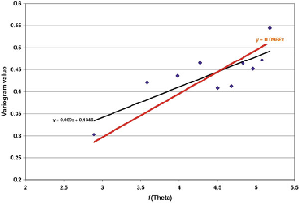
Fig. 6.17 Straight line with equation
y
¼0.0988 ·
x
fitted by constrained least squares to
10 variogram values taken from Matheron (
1962
). Horizontal axis is for
f
(
ʸ
). This line was forced
through the point with
f
(
) ¼0 and
h
¼0. Best-fitting line without this constraint has two
coefficients and is significantly different (Source: Agterberg
2012
, Fig. 8)
ʸ
The preceding experiment illustrates (a) different variogram models applied to
the same data sets can produce similar estimates of extension variances; and
(b) extension variance estimates are too large if there is a “nugget effect” incor-
porating strong autocorrelation over very short distances. In the remainder of this
section it will be attempted to model this type of nugget effect by (a) extrapolation
from the original variogram values, (b) multifractal modeling, and (c) spectral
analysis. The Pulacayo zinc example will be re-analyzed. Because this series
is based on 118 values only, the estimated autocorrelation (or semivariogram)
values have limited precision as previously shown by Agterberg (
1965
,
1967
).
For this reason, autocorrelation for a very large data set was studied as well.
It will be shown (Sect.
6.2.7
) that there is a nugget effect in copper concentration
values from along the deep KTB borehole with short-distance extent that is similar
in consecutive series of 1,000, 1,000 and 796 values, respectively.
6.2.5 Extension Variance
Matheron's geometrical approach can be used for several other purposes. Basic
geostatistical theory (Box
6.7
) results in equations for the extension variance
E
for
the uncertainty associated with using the element concentration value of a small
block as the concentration of a larger block that surrounds it. For example, in
˃
Search WWH ::

Custom Search