Geoscience Reference
In-Depth Information
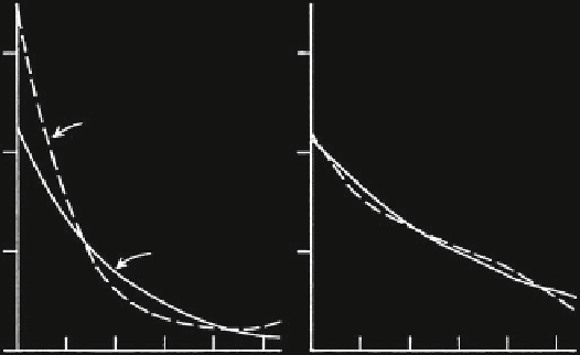
CLAY
SILT
3
3
EXP (CUBIC)
2
2
1
1
EXP (LINEAR)
0
200
400
200
400
TIME IN YEARS
Fig. 6.6 Exponential trends, silt and clay, series 4 (Source: Agterberg and Banerjee
1969
, Fig. 8)
6.1.2 Trend Elimination and Cross-Spectral Analysis
A more detailed time series analysis has been performed of series 4 which,
with 537 varves, covers the longest time interval. First polynomial curve-fitting
was performed on the logarithmically (base
e
) transformed data. Percentages of
explained sums of squares due to linear fits were 43.0 and 38.0 % for silt and clay
thickness data, respectively. These %ESS values were increased to 48.2 and 38.6 %,
after addition of quadratic terms. Further improvements due to cubic fits were small
with %ESS values of 48.5 and 39.5 %, respectively. The linear and cubic exponential
trends are shown in Fig.
6.6
. These curves were obtained by elimination of the
effects of the logarithmic transformation on the trend. In the linear case, this procedure
yields the following exponential curve for thickness in cm:
H
(
t
) ¼ exp {
a
+
bt
+
½
s
2
}
where
H
(
t
) represents the exponential thickness decrease with
t
measured in years,
a
and
b
are constants, and
s
2
is the residual variance (Agterberg
1968
;Heien
1968
). It
represents the solution of the deterministic differential equation:
dH
(
t
)/
dt
H
(
t
). In
Agterberg and Banerjee (
1969
), the dimension of time (
t
) is replaces by that of
distance (
x
) so that the exponential trend curves represent thickness profiles of
individual varves. The preceding two equations then can be written as:
H
(
x
)
¼
¼
exp
(
H
(
x
)
represents the decrease in varve thickness away from the source over a short distance
Δ
cx
)and
dH
(
x
)/
dx
¼
cH
(
x
). It follows that:
Δ
H
(
x
)
¼
cH
(
x
)
Δ
x
where
Δ
x
. Therefore, this model would mean that thickness away from the source is
everywhere proportional to thickness. It provides a fair approximation for the clay,
but for the silt relatively more material was deposited close to the source (Fig.
6.6
).
Refined spectral analysis and cross-spectral analysis can be applied to the residuals
from the linear trends for the log-thickness data (base
e
) of both silt and clay.
The resulting new correlograms are shown in Figs.
6.7
and
6.8
, respectively.
Shifting the series of clay residuals with respect to the series of silt residuals resulted
Search WWH ::

Custom Search