Autocorrelation and Geostatistics - Geomathematics: Theoretical Foundations, Applications and Future Developments - page 195

S A

S

G S S

G S

A

32

16
8
4

1 SERIES 1

B

1

S

2
1
1/2
1/4

A

A

SERIES 2

S

B

A 1

SERIES 3

8
4
2
1
1/2
1/4
1/8
1/16

S SS S B

S S G

S SERIES 4

S
100

300 400 500

B

S

1

A

1/32

8
4
2
1
1/2

SERIES 5

B B

S B

S SERIES 6

1/4
1/8
1/16

B

S

S

I

SERIES 7

S G

S

8
4
2
1
1/2

SERIES 8

100 200 300

TIME IN YEARS

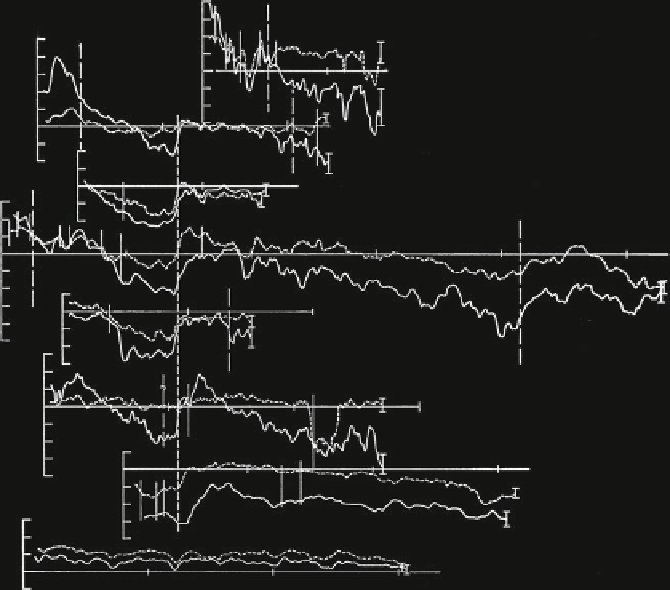
Fig. 6.4 Filtered curves for thickness data, series 1-8. Solid lines denote silt thickness, broken lines
for clay thickness. A-A is boundary between sandy and silty facies, B-B is boundary between silty
and diamictic facies, s slumped intervals, G gaps in record with 5-10 varves missing. Width of 95 %
confidence belt is shown at end of each series (Source: Agterberg and Banerjee 1969 ,Fig.7)

c and a are constants are shown for m 50. Deming's ( 1948 )method

of least squares for exponentials was used for the curve-fitting. Clearly, the
correlogram curves (original data and lines of best fit) intersect the vertical
axis at points that are less than one. This indicates the presence of random
(uncorrelated) noise with variance of standardized data equal to (1

¼ 10 and m ¼

c ). This
white noise can be removed from the data by using the filter of Box 6.2 as
follows.
Application of the semi-exponential filter to series 4, silt, (with m

¼ 10) yielded,

a 0.17 ( cf. Agterberg and Banerjee 1969 )

indicating that the bilateral filter used to derive the relatively smooth “signal” in
Fig. 6.4 is restricted to a relatively narrow neighborhood. Six of the eight series
shown in Fig. 6.4 were aligned with respect to one another on the basis of the
“datum” which is a relatively abrupt increase in thickness of the varves. This datum

¼ 0.022, c ¼ 0.72, p ¼ 0.33 and q ¼