Geoscience Reference
In-Depth Information
radial coordinate is the node number
i
from the com-
putational grid with
r
i
= cos
(iπ/N)
,
i
=1,
...
,
N
,as
described by
Randriamampianina and Crespo Del Arco
[2014] in this topic, which stretches the radial coordinate
to resolve some scales near the boundary. To show the key
distances, the dashed lines indicated the near-wall region,
within 1 and 5% of the gap width and the inner
E
1
/
3
and
outer
E
1
/
4
Stewartson layers. The key regions of variabil-
ity are located in the fluid interior but even more so in
the outer Stewartson layers at the longer time scale of
32 nondimensional time units (
t
=2
t
∗
). This period,
of around 10 rotation periods of the apparatus, is con-
sistent with the usually observed vacillation periods of
structural vacillation. Additionally, there is a source of
much faster fluctuations within the near-wall regions at
a time scale of only three to five time units of the same
magnitude as the rotation period of the annulus. This sug-
gests that a relatively fast boundary layer process might
be involved in the onset of structural vacillation whereas
amplitude vacillation was understood as a global instabil-
ity of the fluid interior. The azimuthal spatial spectrum in
Figure 3.14 shows the clear peaks of the dominant mode 2
and its harmonics superimposed on a general decay with a
decay rate between
p
θ
10
1
10
0
10
-1
-5/3
∝
k
10
-2
10
-3
10
-5
10
-4
10
-3
k
r
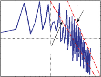
Figure 3.15.
Radial spatial spectrum averaged over time and
azimuth for structural vacillation.
still steady fundamental radial mode of that wave, is
supported by the experiments of
Früh and Read
[1997]
and explained in a low-order Eady-type model by
Weng
et al.
[1986]. This explanation would suggest that there
is a clear bifurcation route from the steady wave to the
AV, which then bifurcates to a SV in some way. How-
ever, this bifurcation remains elusive, and calculations of
the Grassberger-Procaccia dimension of amplitude vacil-
lations and structural vacillations have repeatedly shown
that amplitude vacillations are well behaved and appear to
follow low-dimensional dynamics whereas the dimension
estimates for measurements from structural vacillations
do not converge to a reliable estimate [
Guckenheimer and
Buzyna
, 1983;
Read et al.
, 1992;
Früh and Read
, 1997].
Another explanation might be a localized instability of
the large-amplitude wave resulting in possibly a barotropic
instability of the type of a detached shear layer [
Früh
and Read
, 1999] but localized in space along the edges of
individual wave lobes or in the form of a breaking wave
leading to internal gravity waves such as those described
by
Jacoby et al.
[2011]. Yet another option might be a
boundary layer instability as the large-amplitude wave
impinges on the sidewalls, such as seen by
Read et al.
[2008] and
Früh et al.
[2007].
m
−
2.2
and
m
−
3
, which would be
consistent with a quasi-geostrophic turbulence spectrum
[
Charney
, 1971;
WaiteandBartello
, 2006]. The radial spec-
trum in Figure 3.15, on the other hand, has a spectrum
with radial wave number as
p
r
∼
∼
k
−
5
/
3
, which is closer
to a mesoscale energy spectrum in terms of the horizontal
wave number [
Nastrom and Gage
, 1985] or strongly strat-
ified turbulence where strong small-scale static instability
is present [
Lindborg
, 2006].
One suggested route, the instability of a higher radial
mode of the dominant wave growing to a finite-amplitude
modulation of that higher mode superimposed on the
10
0
-3
∝
m
10
-1
-2.2
∝
m
3.7. AMPLITUDE VACILLATION AS STEP
TOWARD CHAOS AND TURBULENCE
10
-2
10
0
In this context, the distinction between “chaos” and
“turbulence”is based on the assumption that chaotic flow
is governed by deterministic equations that can be mod-
eled by a finite (hopefully small) number of degrees of
freedom whereas turbulence requires so many dimensions
10
1
10
2
m
Figure 3.14.
Azimuthal spatial spectrum averaged over time
and radius for structural vacillation.