Geoscience Reference
In-Depth Information
(a)
(b)
A
Z
→
0.25
0.8
A
E
→
K
E
0.2
0.6
0.15
A
Z
→
A
E
0.4
←
A
E
0.1
0.2
K
E
→
K
Z
K
Z
0.05
K
E
0
A
Z
→
K
Z
0
−0.2
400
500
600
700
800
900
1000
1000
400
500
600
700
800
900
Time (s)
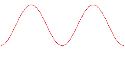
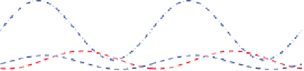
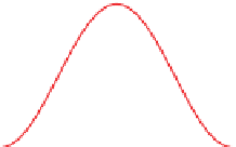
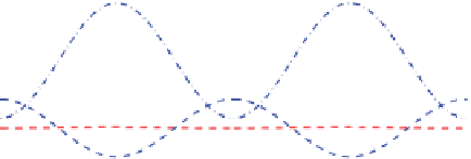
Figure 3.5.
Idealization of the energetics for an amplitude vacillation cycle (after
Pfeffer et al.
[1973]) using
A
Z
for zonal potential
energy,
A
E
for eddy potential energy,
K
E
for eddy kinetic energy, and
K
Z
for zonal kinetic energy: (a) energy contained in that type
and (b) rate of energy transfer from one type to another. Adapted from Figures 17, 18, and 19 of
Pfeffer et al.
[1973]. Copyright ©
American Meteorological Society. Used with permission.
observation that vacillating flows occurred on increasing
the rotation rate (or the forcing toward favoring higher
wave numbers). At the time this was surprising as all
previous vacillation studies had been carried out in liq-
uids where vacillation is found on decreasing the rota-
tion rate.
Randriamampianina et al.
[2006] then traced a
full bifurcation sequence from the initial instability to a
chaotic modulated amplitude vacillation that was subse-
quently confirmed experimentally by
Castrejon-Pita and
Read
[2007].
F
F
D
Z
K
Z
A
Z
D
Z
K
Z
A
Z
D
E
K
E
A
E
D
E
K
E
A
E
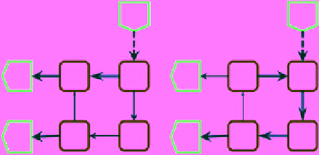
Low-amplitude wave
Large-amplitude wave
Figure 3.6.
Schematic of the energy flow during the two
extreme stages of an amplitude vacillation as calculated by
Pfeffer et al.
[1973] using
F
for forcing,
A
Z
for zonal potential
energy,
A
E
for eddy potential energy,
K
E
for eddy kinetic energy,
K
Z
for zonal kinetic energy, and
D
for dissipation. Adapted from
Figures 20 and 21 of
Pfeffer et al.
[1973]. Copyright © American
Meteorological Society. Used with permission.
3.3.2. Quasi-Geostrophic Approximation
In the quasi-geostrophic approximation, the momen-
tum equations are scaled against the Coriolis term and
then ordered in a series of terms of increasing power of
the Rossby number, where the Rossby number is the ratio
of the advection term to the Coriolis term, Ro =
U/(fL)
[e.g.,
Pedlosky
, 1987]. If the Rossby number is small, the
leading balance of forces is the Coriolis force to the hori-
zontal pressure gradient, which leads to the definition of
the geostrophic stream function. The terms of
O(
Ro
2
)
then give an equation for the evolution, advection, and
diffusion of this geostrophic stream function.
Based on the quasi-geostrophic approximation, a vari-
ety of models have been developed, all of which center
around wave mode perturbations for the horizontal
motion around an idealized baroclinic basic state. The
vertical structure of this baroclinic basic state could be
continuous, such as the Eady model [
Eady
, 1949] or
the Charney model [
Charney
, 1949], or discrete, such as
Phillips' two-layer model [
Phillips
, 1951]. The model can
be used for high-resolution modeling for a systematic
truncation to a low order or for investigating the evolution
of a specific perturbation.
observed that the amplitude vacillation showed a clear
oscillation of the relative phase of the wave in the lower
part of the annulus compared to that of the upper part.
Steady baroclinic waves have long been associated with a
clear westward tilt of the temperature field and associated
vertical heat transport [e.g.,
Hide and Mason
, 1975]. With
this in mind, the strong variation in the westward tilt is
associated with the transfer between eddy kinetic energy
(little tilt) and eddy potential energy (strong tilt) from the
basic energy transfer model given in Figure 3.4. In con-
trast, the case classified as structural vacillation shows
no such vertical tilt of the flow features but is essentially
barotropic.
A high-resolution spectral Fourier-Chebyshev model of
the thermal annulus filled with air was used by
Maubert
and Randriamampianina
[2002] with the then-surprising