Geoscience Reference
In-Depth Information
A
corresponds to a relative change in value of
b
and
c
such
that the line
μ
2
=
of case VIIa [
Guckenheimer and Holmes
, 1983]. This case
is presented as “difficult” case I by
Kuznetsov
[2004]. In
this case, there is a supercritical Hopf bifurcation at
μ
2
=0
and a subcritical Hopf bifurcation at
μ
1
= 0. The subcrit-
ical Hopf bifurcation indicates that there is an unstable
periodic orbit for negative values of
μ
1
. Such a bifurcation
is associated with a hysteretic primary transition. How-
ever, the hysteresis occurs via a different mechanism than
the hysteresis observed in the wave regime. In particular, if
it is assumed that there is a smooth transition between the
supercritical and subcritical cases, we can assume that the
branch of stable wave solutions of wave number
m
j
that
exists in the wave regime (i.e., for positive values of
μ
j
)in
the supercritical case does not disappear. Thus, the branch
of unstable wave solutions that emanate from the subcrit-
ical Hopf bifurcation will link up with the stable branch
in a saddle node bifurcation at some negative value of
μ
j
,
creating a region in parameter space in which the stable
axisymmetric solution and stable wave solutions coexist.
This creates the necessary conditions to observe hystere-
sis. The analysis presented here, i.e., the computation of
only the third-order coefficients, is insufficient to prove
whether this actually occurs or to determine the extent of
the hysteresis (i.e., the parameter value at which the sad-
dle node bifurcation occurs). The higher order coefficients
may be able to determine these. However, even the compu-
tation of the coefficients of the next order is prohibitively
difficult, and so we do not compute it here. In Section 2.5,
we discuss alternative methods that are capable of com-
puting both the stable and unstable branches and there-
fore of showing the existence and extent of the hysteresis.
Hysteretic transitions have been observed in the numeri-
cal experiments of
Randriamampianina et al.
[2006] in the
case of a near-unity Prandtl number fluid. However, the
range of hysteresis is very small, which may account for
why it is not observed in the experiments of
Castrejon-Pita
and Read
[2007]. Hysteresis is also observed in the case
of higher Prandtl number fluid when the upper surface of
the fluid is free [
Fein
, 1973]. Figures 2.2-2.4 all indicate
that such hysteretic transitions become more common at
lower Prandtl number, first appearing at Prandtl number
less than 3, in the
(m
1
,
m
2
)
=
(
3,2
)
mode interaction.
However, the figures do not indicate the largest value of
the Prandtl number at which hysteresis occurs because
the mode interaction points only provide information at
a single point on the transition curve. The other mode
interaction points show a hysteretic primary transition at
much lower values of the Prandtl number. We also note
that Case VIIa, subcase (b) occurs in the
(m
1
,
m
2
)
=
(
4,3
)
mode-interaction point at Prandtl number correspond-
ing to that of air. However, this nor any of the other
Cases observed for these parameters explain the occur-
rence of the experimentally observed weak waves, see
[
Castrejon-Pita and Read
, 2007;
Lewis
, 2010].
cμ
1
.
Because the fixed points 2 and 3 are stable under the
same conditions, they are both now
unstable
in the wedge
defined by
μ
2
<
−
μ
1
/b
now lies above
μ
2
=
−
cμ
1
. Linear stability
analysis of fixed point 4 reveals that it is now always
stable
when it exists. Thus, the mixed-mode flow corresponding
to fixed point 4 may be observable in experiment. The
two-parameter bifurcation diagram is presented as simple
case 2 by
Kuznetsov
[2004]; it has a similar structure as in
Figure 2.5, except with the change in relative orientation
of the lines
μ
2
=
−
μ
1
/b
and
μ
2
>
−
cμ
1
and the change
in stability of the fixed points as indicated.
Subsequently, for all mode interaction points, a decrease
in Prandtl number leads to a change in sign of the coef-
icient
c
, which implies that
A >
0.Thus,wehavecase
II
, which is the time reverse of case II of
Guckenheimer
and Holmes
[1983].
Kuznetsov
[2004] refers to this as sim-
ple case 3. See Figure 2.7. This is similar to case Ia
except
that the line
μ
2
=
−
μ
1
/b
and
μ
2
=
−
cμ
1
now lies below the line
μ
2
=0.
As above, the negative
a
and
d
indicate that there exist
periodic orbits corresponding to fixed points 2 and 3 for
μ
1
>
0and
μ
2
>
0, respectively, and fixed point 4 exists
in the wedge defined by
μ
2
<
−
cμ
1
.
Linear stability analysis reveals that fixed points 2 and 3
are stable (unstable) outside (inside) this wedge, when they
exist, and that fixed point 4 is always stable. Thus, again
the mixed-mode flow corresponding to fixed point 4 may
be observable in experiment.
Again, for all mode interaction points, as the Prandtl
number is decreased, there is a transition to case VIIa. In
this case, we have
a
=1,
b <
−
μ
1
/b
and
μ
2
>
−
1, and
A >
0.
For most instances when this case applies, we also have
that
b <
−
1,
c >
1,
d
=
−
−
1and
c >
1, which corresponds to subcase (b)
μ
2
ρ
2
μ
2
=-
μ
1/
b
ρ
1
μ
1
μ
2
=-
c
μ
1
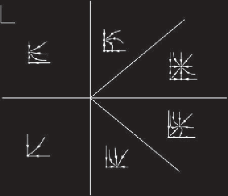
Figure 2.7.
Two-dimensional bifurcation diagram for case II
.
See caption of Figure 2.5 for description.