Geoscience Reference
In-Depth Information
(a)
(b)
VIa
VIb
Ib
II
′
4
5
a
b
c
d
A
Ia
′
Ib
VIa
V
VIIa
Ib
′
2
II
0
0
-2
-5
0.1
0.2
0.3 0.4
Prandtl number Pr
0.5
0.6
0.7
2
4
6 8
Prandtl number Pr
10
12
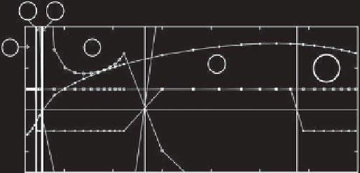
Figure 2.2.
Results for the
(m
1
,
m
2
)
=
(
3, 2
)
mode interaction point. Computed values of the normal form coefficients
a
,
b
,
c
,
and
d
and
A
=
ad
bc
are shown as a function of the Prandtl number Pr. (a) Results for Pr between 0.025 and 0.7 and (b) results
for Pr between 0.7 and 13, where at Pr = 0.025 the parameters correspond to those of mercury, at Pr = 0.7 to those of air, and
at Pr = 13 to those of a water-glycerol mixture. In order to ensure that the values of
ν
and
κ
correspond to those of these fluids
at the given Prandtl number, it is necessary to change the magnitude of the incrementation of
ν
and
κ
as the Prandtl number is
varied; discontinuous changes in the incrementation result in kinks in the graphs of
b
,
c
,and
A
. Vertical lines indicate transitions
between qualitatively different dynamics that are labeled according to the case numbers of
Guckenheimer and Holmes
[1983].
−
(a)
(b)
VIa
VIb
4
5
a
b
c
d
A
Ia
′
II
V
VIIa
Ib
′
III
II′
2
VIIa
0
0
-2
-5
0.1
0.2
0.3 0.4
Prandtl number Pr
0.5
0.6
0.7
2
4
6
8
10
12
Prandtl number Pr
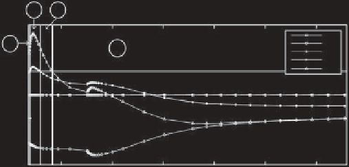
Figure 2.3.
Results for the
(m
1
,
m
2
)
=
(
4, 3
)
mode interaction point. See caption of Figure 2.2 for description.
(a)
(b)
VIb
II
′
Ia
′
VIIb
VIa
2
b
d
A
4
Ia
′
Ib′
VIIa
II
′
2
0
0
-2
-2
-4
-4
0.1
0.2
0.3 0.4
Prandtl number Pr
0.5
0.6
0.7
2
4
6
Prandtl number Pr
8
10
12
Figure 2.4.
Results for the
(m
1
,
m
2
)
=
(
5, 4
)
mode interaction point. See caption of Figure 2.2 for description.