Geoscience Reference
In-Depth Information
(b)
(a)
Temperature - 22.000000 (°C)
Temperature - 22.000000 (°C)
8
8
6
6
4
4
2
2
0
0
t
= 10500.000 s
t
= 1185.0000 s
-2
-2
-4
-4
-6
-6
-8
-8
-8
-8
-6
-4
-2
0
2
4
6
8
-6
-4
-2
0
2
4
6
8
x
(cm)
x
(cm)
-1.2e+00
-9.0e-01
-6.0e-01
-3.0e-01
0.0e+00
-2.0e+00
-1.5e+00
-1.0e+00
-5.0e-01
0.0e+00
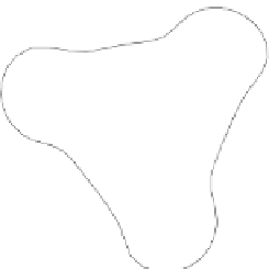
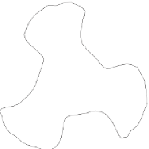
Figure 1.27.
Representative temperature fields (colors) and horizontal stream function (contours) produced from assimilated
horizontal velocity observations obtained in the same system as shown in Figures 1.8-1.13 and 1.21-1.26. Fields are plotted
for regular (a)
= 0.875 rad/s,
T
b
−
4.02
◦
C) at
z
= 9.7 cm above the
base of the annulus. Temperatures are relative to 22
◦
C. Adapted from
Young and Read
[2013] with the permission of John Wiley
& Sons, Inc. For color detail, please see color plate section.
4.07
◦
C) and chaotic flow (b)
=3.1rad/s,
T
b
−
T
a
≈
T
a
≈
atmosphere and oceans, offering the same potential uses
to (a) obtain analyses of complete fields in the presence of
incomplete and noisy measurements, (b) enable determin-
istic model predictions from assimilated measurements to
quantify predictability and sensitivity to initial conditions,
and (c) identify, characterize, and quantify systematic
model errors.
The work by
Young and Read
[2013] applying data
assimilation to the rotating annulus experiment in the
form of analysis correction [
Lorenc et al.
, 1991] began to
address some of these points. They demonstrated that it
is possible to take methods developed for meteorological
analysis and prediction and use them in the context of the
laboratory experiment toward a useful end. In particular,
they addressed the problem of incomplete measurements
using the analysis correction procedure with a Boussi-
nesq Navier-Stokes model to recover unobserved variables
such as temperature (Figure 1.27) solely from irregularly
distributed horizontal velocity observations at five verti-
cal levels. The diagnostics required to shed light on the
secondary instabilities at high rotation rate described in
Section 1.3.4 were only obtainable because unobserved
variables and vertically averaged quantities were retrieved
via the assimilation procedure.
Although they did not address any outstanding prob-
lems with the analysis correction method itself (it has
since been superseded by newer methods), this work laid
the foundations to do so with newer methods not yet
fully established in operational meteorological practice.
Potential methods of interest include the various fla-
vors of the ensemble Kalman filter (a version of which
Ravela et al.
[2010] have applied in this context) and other
experimental methods that have been tested thus far pri-
marily using low-dimensional systems [e.g.,
Stemler and
Judd
, 2009;
van Leeuwen
, 2010]. Laboratory experiments
bridge the gap between these low dimensional systems
and geophysical systems such as the atmosphere and,
by using laboratory experiments, methods can be tested
under laboratory conditions using a real fluid, a nonideal-
ized model, and incomplete and noisy observations.
1.5.1. Planetary Circulation Regimes
An important question that still deserves a lot more
attention than has been evident in the literature to date
is the extent to which the rich and complex diversity of
different flow regimes and bifurcations exhibited in the
laboratory are shared, even qualitatively, by a full scale
planetary atmosphere. The inability to carry out con-
trolled experiments on real atmospheres is a major obsta-
cle to progress in this regard (although of course such an
approach would have other undesirable consequences for
the inhabitants of such a planetary system!). The solar
system provides a small sample of around eight plane-
tary bodies with substantial atmospheres that occupy very
different positions in parameter space. But this samples