Geoscience Reference
In-Depth Information
(a)
(b)
(c)
160
140
120
100
80
60
40
20
150
0.01
150
0.015
0.01
0.005
0
-0.005
-0.01
-0.015
-0.02
0.01
0.005
100
100
0
0
-0.005
50
50
-0.01
-0.01
-0.02
20
40
60
80 100 120 140 160
50
100
150
50
100
150
(d)
(e)
150
150
5
0.01
100
100
0
0
-0.01
50
50
-5
-0.02
-10
50
100
150
50
100
150
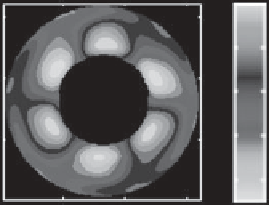
Figure 17.12.
Experiment with parameters
=6rpm,
T
= 8 K. (a) EOF1, 27% explained variance. (b) POP1, damping time
1827.6 s, period 62.5 s. (c) First singular vector at
t
=0,
t
opt
=20s,
σ
= 1.182. (d) First singular vector at
t
=
t
opt
. (e) First singular
vector at
t
= 2500 s.
The starting point for the SV analysis is the linear
dynamical system
low-dimensional systems [
Harlander et al.
, 2009a] but it
fails in general.
Having estimated the system matrix
B
from (17.12), we
can compute the propagator
G
for any time interval
0
by
d
x
dt
=
Bx
(17.10)
with the system matrix
B
. In atmospheric ensemble pre-
diction linearization is generally done around a nonlinear
solution and then
B
is time dependent. In contrast, in
turbulence research linearization is done around a mean
state. In that case
B
is time independent [
DelSole
, 2007].
We consider the mathematically simpler latter case.
The matrices
G
in (17.7) and
B
in (17.10) are connected
via the equation
G
()
= exp
(
B
)
=
∞
G
(
0
)
= exp
(
B
0
)
.
(17.14)
When the
L
2
-norm is used to measures the growth of a
perturbation in the time interval 0
0
, the SVs with
optimazation time
0
are given by the eigenvectors of
the matrix
G
T
(
0
)
G
(
0
)
. The eigenvalues of the matrix
define the square of the growth rates.
Figure 17.12c shows the first singular vector at
t
=0
estimated from surface temperature data of an experiment
with
=6rpmand
T
= 8K. The data sampling rate
was
= 5 s, and the optimization time was set to be
0
=
20 s. For the time interval 0
≤
t
≤
1
k
(
B
)
k
(17.11)
!
k
=0
or
0
we obtain a growth
rate of
σ
= 1.182. To reduce the noise in the data, we used
the EOF filtering technique. Just 33 EOFs explain a total
variance very close to 90%. Thus we used
j
= 33 in (17.5)
to reconstruct the data from the EOFs. It should be noted
that the growth rate increases by increasing the number of
EOFs used for the reconstruction. It appears that the more
EOFs that are available to support the SVs, the larger is the
maximum growth rate. However, reconstructing the data
by a large number of EOFs increases the noise, and at a
certain number, the SVs seem to be dominated by noise
and lose their physical meaning.
≤
t
≤
∞
1
)
k
+1
k
B
=
1
=
1
(
−
k
, (17.12)
ln
[
G
()
]
[
G
()
−
E
]
k
=1
where
E
is the identity matrix. It is instructive to note that
by discretizing the first term in (17.10) by
[
x
(t
+
)
−
x
(t)
]
/
and using (17.6), we find
B
=
1
[
G
()
−
E
]
.
(17.13)
This corresponds to (17.12) when just the first term
is kept. The simplification gives still good results for