Geoscience Reference
In-Depth Information
x10
-3
8000
7000
6000
5000
4000
9
8
7
6
5
4
3
2
1
0
10
3000
2000
1000
0
1
0,1
02468 0
Rank
2
4
6
8
10
12
14
16
18
20
12
14
16
18
20
x10
-3
x10
-4
8000
7000
6000
5000
4000
3000
2000
1000
0
8000
7000
6000
5000
4000
3000
2000
1000
0
1
4
2
0
-2
-4
-6
0.5
0
-0.5
-1
Azimuth
Φ
=0-2
π
Azimuth Φ =0-2π
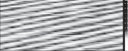
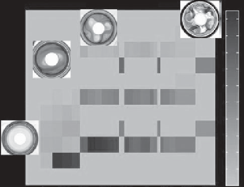
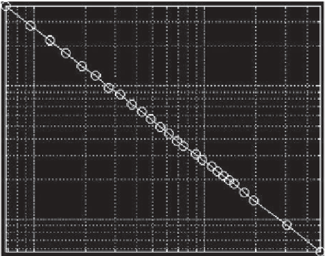
Figure 17.5.
MSSA analysis of a wave mode of dominant wave number
m
= 4. Upper left: Space-time plot of the homogenized
LDV data set, radial velocity [m
/
s] over azimuth 0
2
π
. Upper right: The first 20 eigenvalues of the MSSA covariance spectrum.
Note that a logarithmic scale has been used. Lower left: Reconstructed space-time plot using the first two MSSA eigenvectors.
Lower right: Reconstructed space-time plot using the third and the fourth MSSA eigenvectors.
−
(a)
(b)
Variance of EOFs
12
m
=2
50
45
10
m
=3
40
10
0
35
8
30
25
6
20
15
10
-1
10
m
=4
2
5
10
7
10
8
7
7.2
7.4 7.6 7.8
Log Taylor number
8
8.2
8.4
8.6
Ta
Figure 17.6.
EOF variance spectra obtained along a transection through the wave regime. Left: Each circle in the Ta Rodiagram
corresponds with an experiment. Right: Distribution of the variance (in % of the total variance) for the first 12 wave modes as a
function of Ta. See also Table 17.1. For color detail, please see color plate section.
(
m
= 6,9) in the EOF variance spectrum. When we
increase Ta, the dominant wave becomes weaker and the
first harmonics stronger. At the transition to
m
=4(at
(
Ta, Ro
)
=
(
3.04
to identify a dominant wave. The EOF variance spectrum
starts to become broader. Within the
m
= 3 regime we find
transitions to the
m
= 4 flow indicating regions of multiple
equilibria. Note that the irregular wave flow must not be
confused with turbulent flow. For the first a wave pattern
is still present whereas for the latter it is not.
10
−
2
)
) the first harmonic
comprises as much variance as the
m
= 4 mode. The flow
is rather irregular and it becomes more and more difficult
10
8
,9.01
×
×