Geoscience Reference
In-Depth Information
°C
°C
°C
25
25
25
24
24
24
23
23
23
22
22
22
t
=+1200 s
t
=+3000 s
t
=0s
°C
°C
°C
25
25
25
24
24
24
23
23
23
22
22
22
t
=+30s
t
=+60s
t
=+90 s
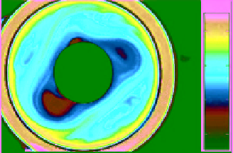
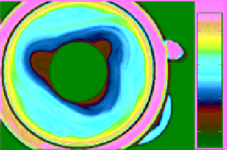
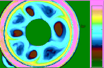
Figure 17.3.
Sequence of thermographic measurements describing vacillating flows [
von Larcher and Egbers
, 2005b]. Top: Wave
mode competition of wave number
m
=2and
m
= 3 at Ta = 1.08
10
7
, Ro = 3.00. Bottom: Structural vacillation flow, radial
×
10
7
, Ro = 0.41, with
t
as relative time.
oscillation of a wavy flow of wave number
m
= 4 at Ta = 7.65
×
and Zwiers
, 1999] that reveals propagating patterns of
variability by single CEOFs, whereas pure EOFs capture
only standing modes of variability.
The MSSA is a generalization of the single-time-series
SSA method to multiple time series [
Broomhead and King
,
1986;
Read
, 1992;
Vautard
, 1995]. These time series may
contain observations of a certain variable at different loca-
tions (as in our case) or even observations of different
variables. In classical EOF analysis the dominant spa-
tial patterns are captured by diagonalizing the covariance
matrix. As discussed
Vautard
[1995], the coordinates of
the state vector in the EOF analysis represent different
locations in space at the same time. In an SSA, the state
vector contains values at the same locations but at dif-
ferent time lags. CEOF analysis is a special case of the
MSSA method; however, MSSA deals with more tem-
poral degrees of freedom than spatial ones, allowing the
investigation of spectral properties of the data. In con-
trast, CEOF contains only a single lag but a large number
of spatial points. The MSSA method allows one to detect
oscillating features in noisy time series where oscillations
occur frequently only during certain time periods. The
larger generality of the MSSA is purchased by a larger
amount of computing time. A detailed description of the
MSSA method is beyond the scope of the present chapter
but is given by
Dettinger et al.
[1995],
Vautard
[1995], and
Elsner and Tsonis
[1996].
POPs are empirical, that is, data estimated normal
modes [
Hasselmann
, 1988]. POPs are another way of
decomposing a data set into a signal and noise subspace.
To evaluate POPs, the system matrix corresponding to a
linear model has to be found as described, e.g., by
von
Storch and Zwiers
[1999]. Frequently, POPs correspond
with EOFs, though this correspondence is not guaranteed
from a mathematical point of view. Also the correspon-
dence between true normal modes and POPs is not always
obvious [
J.-S. von Storch
, 1995]. In real data, linearly
unstable modes occur only in a nonlinearly saturated state.
Thus POP modes are either neutral or damped. In con-
trast, a linear operator might allow for unstable modes
that cannot be covered by any data based method. Nev-
ertheless, POP analysis has proven to be useful in a broad
range of applications and can be considered as one of
the routine tools in climate research. From the empirically
estimated system matrix, not only POPs can be computed.
A further useful step is to estimate SV, from the system
matrix. SVs correspond to those initial perturbations that
grow in an optimal sense with respect to a chosen norm
within a predefined time interval, the so-called optimiza-
tion time. For large-scale baroclinic systems, SVs might
play an important role and they might be even more rel-
evant for real flows than unstable normal modes [
Badger
and Hoskins
, 2001].
All the four mentioned orthogonal decompositions
(EOF analysis, MSSA, POP analysis, SV analysis) are
related via the data matrix. Let us briefly describe how. A
variable
X
i
is observed at
M
different arbitrarily spaced
points,
i
=1,2,
...
,
M
,andat
P
different instances of