Geoscience Reference
In-Depth Information
Receiver
(a)
-40
Measurement
volume
V
scat
r
-60
Nozzle
q
scat
n
Tranquilization
chamber
Jet flow boundaries
-80
Transmitter
-100
-4000
-2000 0
Doppler frequency (Hz)
2000
4000
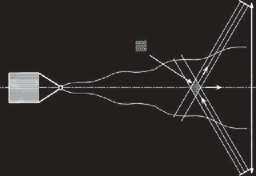
Figure 15.15.
Example of implementation of vorticity measure-
ment by acoustic scattering in a turbulent jet. From
Poulain et al.
[2004]. Note that the same configuration can be easily ported
to open flows and in city measurements in the atmospheric
boundary layer.
(b)
10
4
K41: slope 1/3
10
3
1999]). Figure 15.15 shows the schematic of the implemen-
tation of acoustic measurement of vorticity in a turbulent
jet as done by
Poulain et al.
[2004]. In this experiment
acoustic transducers are of Sell type consisting of a cir-
cular plane piston, with typical diameter of the order of
10 cm (larger and smaller transducers can be used depend-
ing on the extent of the flow to be probed), made of a
thin mylar sheet (typically 15
μ
m thick). One important
advantage of such transducers is their large bandwidth
(typically between 1 and 200 kHz in air) which allows to
span a wide range of scattering wave vectors
η
η
10
2
2π
2π
L
int
λ
10
10
-3
10
-2
10
-1
1
q
scat
η
q
scat
with
a fixed geometric arrangement (in particular with a fixed
scattering angle). In the example, the scattering angle was
kept fixed at constant value of the order of 60
◦
.The
choice of the working scattering angles responds to several
criteria: (i) Given the angular factor dependence shown
in Figure 15.14, angles close to 90
◦
and 180
◦
should be
avoided. (ii) At small scattering angles the angular factor
increases rapidly; however, unless thermal conditions in
the experiment are very well controlled small scattering
angles should be avoided as forward sound scattering is
very sensitive to temperature gradients. (iii) Other prac-
tical criteria include, for instance, geometric constraints
around the experiment, limitation of echoing effects and
direct acoustic “blinding” from the emitter to the receiver
(in particular via the secondary diffraction side lobes
of the transducers). (iv) Beyond these practical consid-
erations, the scattering angle should also be chosen in
accordance with the physical properties of the flow to be
probed. As already discussed, the amplitude of the scat-
tering vector
q
scat
=4
πν
0
/c
sin
(θ
scat
/
2
)
defines the wave
number at which the vorticity spectrum is being probed. It
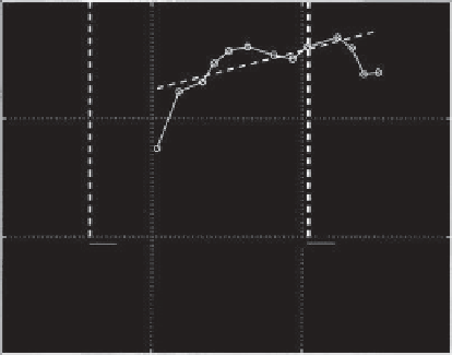
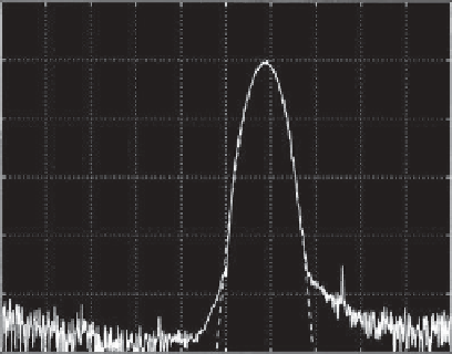
Figure 15.16.
(a) Power spectral density of the signal scattered
by the flow. (b) Discrete reconstruction of the spatial spectrum
of the flow enstrophy. From
Poulain et al.
[2004].
can be selected by changing either the working frequency
or the scattering angle. Hence, the scattering angle will be
chosen so that wave numbers relevant to the investigated
problem can be effectively spanned within the accessible
range of operating frequencies of the acoustic transduc-
ers. In our case, an angle of 60
◦
allowed the authors to
probe a significant range of the inertial scales of the turbu-
lent jet with a constant scattering angle by simply varying
the working frequency
ν
0
of the transducers.
As an example of results which can be obtained with
this technique, we show in Figure 15.16a a typical power
spectrum of the signal recorded by the acoustic receiver
(note that the signal has been down-mixed exactly in the
same way as explained for the acoustic Lagrangian mea-
surement in the previous section). The maximum of the
power spectrum occurs for a nonzero frequency which