Geoscience Reference
In-Depth Information
-0.5
-0.6
-0.7
-0.8
0.005
0.01
0.015
0.02
0.025
0.03
Time (s)
0.04
0.02
0
-0.02
-0.04
0.014
0.0145
0.015
0.0155
0.016
0.0165
0.017
0.0175
0.018
0.0185
0.019
Time (s)
1
0.5
0
-0.5
-1
0.014
0.0145
0.015
0.0155
0.016
0.0165
0.017
0.0175
0.018
0.0185
0.019
Time (s)
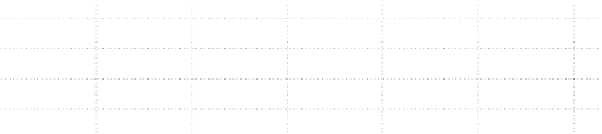
Figure 15.6.
Typical optical signal measured with extended laser Doppler velocimetry. Top: Burst observed when a particle
crosses the measurement volume. Middle: Real part of the complex signal obtained after filtering and demodulation from carrying
frequency
δf
= 100 kHz. Bottom: Corresponding evolution of velocity as obtained from parametric estimation.
Signal Acquisition
The use of two AOMs instead of
one (for classical LDV) allows for a small frequency shift
(100 kHz) so that raw data can be acquired using high-
speed data acquisition board. Each time a particle crosses
the measurement volume, it produces a burst of light with
a signal of the following form (Figure 15.6a):
signals
(s
i
(t))
[
1,
N
]
. This signal processing step is crucial
as both time and frequency, i.e., velocity, resolutions
rely on its performance. As the local frequency of the
signal is varying in time, common time-frequency tech-
niques based on Fourier analysis [
Flandrin
, 1998] (such
as
short-time Fourier transform
) are usually too limited
as the Heisenberg principle imposes that time resolution
δ
t
and frequency resolution
δ
ν
must comply the inequal-
ity
δ
t
δ
ν
>
1, which means that one cannot have both high
resolution in time (which is crucial to resolve the fastest
dynamics of the particles) and frequency (which is crucial
to have a good measurement of particle velocity, which
according to relation (2) is directly given by
ν(t)
). It is
therefore necessary to overcome the Heisenberg princi-
ple limitation. Several methods exist, including Cohen
class energetic estimators (such as Wigner-Ville and Choï
Willians distributions) [
Flandrin
, 1998] which can be fur-
ther refined using the
reallocation
technique [
Flandrin
,
1998;
Kodera et al.
, 1976]. These methods are relatively
time consuming in terms of computational processing and
are generally adapted for situations where no information
is a priori known on the form of the signal to be analyzed.
In order to increase the frequency resolution with a small
observation window, Mordant and coworkers introduced
a fast demodulation algorithm with parametric estima-
tion [
Mordant et al.
, 2002, 2005]. It relies on a comparison
s(t)
=
α(t)
+
β(t)
cos
[
2
πδf
·
t
+
φ(t)
]
,
(15.1)
with
dφ(t)
dt
=2
π
u
(t)
a
⊥
,
(15.2)
where
α(t)
and
β(t)
are slowly varying envelopes originat-
ing from the Gaussian radial profiles of the beams.
1
2
π
dφ(t)
dt
ν(t)
=
.
The Doppler shift of the scattered signal due to the
motion of the scatterer particle is represented as. In a typ-
ical situation, the diameter
d
of the beams is much larger
than the fringe spacing
a
so that there is a scale separation
between the fast modulation at frequency
ν(t)
=
u
(t)/a
⊥
and the slow amplitude modulations
α(t)
and
β(t)
.
Signal Processing
After running the experiment, the
velocity is computed from the collection of light scattering