Geoscience Reference
In-Depth Information
(a)
(b)
10
−1
10
−4
2
2
∼
Δ
r
∼
Δ
r
10
−5
10
−2
t
=40
t
=40
t
=80
10
−6
t
=80
10
−3
t
= 120
t
= 120
t
= 160
t
= 160
10
−7
10
−3
10
−2
10
−3
10
−2
Δ
(m)
Δ
ρ
(m)
ρ
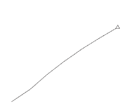
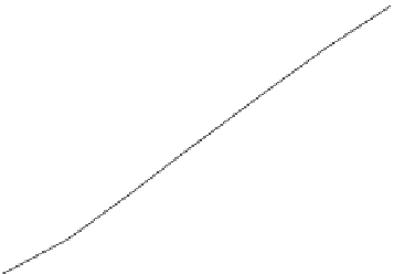
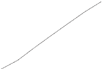
Figure 12.6.
Verification of the numerical scheme described in Section 12.6 for the test case
f
= 1.5 rad
/
s,
f
=0.02rad
/
s. The
pointwise
2
error is plotted in (a) the PV and (b) the stream function between each solution and an “exact” solution is obtained
via Richardson extrapolation.
(a)
(b)
(c)
(d)
(e)
(f)
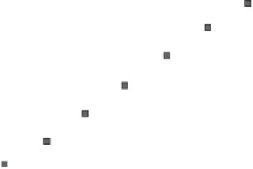
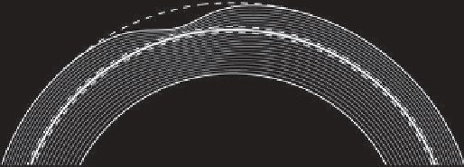
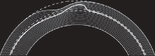
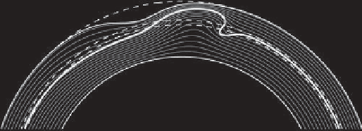
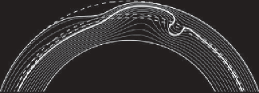
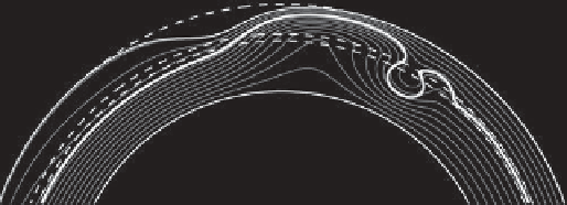
Figure 12.7.
Evolution of the numerical solution of the QG model described in Section 12.5, at (a)
t
= 0 s, (b)
t
=17s,(c)
t
=29s,
(d)
t
=45s,(e)
t
= 66 s, and (f)
t
= 104 s. The numerical parameters have been chosen to match the reference experiment shown in
Figure 12.3. In each snapshot is plotted the position of the passively advected line of tracer (thick black line) and the instantaneous
streamlines with a separation of 2 cm
2
/
s (thin gray lines). The thin black lines show the positions of the inner and outer walls of
the annulus, and the dashed lines highlight the extent of the slope and the width of the protrusion.