Geoscience Reference
In-Depth Information
(a)
(b)
Time (s)
0
1000
2000
3000
4000
5000
6000
700
0
2π
7
6
3
2
5
4
π
3
2
2
1
0
0
1000
2000
3000
4000
5000
6000
7000
0
20
40
60
80
100
120
Number of revolutions (
Phase
2π
)
Time (s)
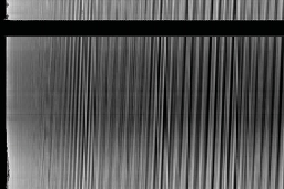
Figure 11.4.
Amplitude vacillation of the baroclinic mode 2 shown in a Hovmöller diagram (a) with maxima at approximately
35, 70, and 100 rotation periods (
x
axis) and (b) the time evolution of the amplitude of the spatial Fourier mode 2. Experimental
parameters:
d
= 0.023, 1
/
Bu =
F
= 3.27.
this period can clearly be seen. This variation is most likely
due to the gradual variation in stratification after more
than 100 rotation periods. This confirms the occurrence
of amplitude vacillation in two-layer miscible fluids with
a smooth interface.
counted. However, due to the interaction between modes,
the structure appears not as regular as the linear predic-
tion. A square lower mode structure can be observed on
top of the Rossby mode that resonates with the Kelvin
mode. Indeed, the temporal evolution of the mode ampli-
tudes reveals that beyond the predominant modes 6 and
5, lower modes (2 and 3) are competing, thus confirming
a nonlinear interaction between modes (see Figure 11.6).
This may explain the observation of much higher growth
rates than the growth rates predicted by the linear theory
[
Gula et al.
, 2009a]. The general structure is nevertheless
in good agreement with the RK instability (Figure 11.5
left side) (Gula, personal communication; see also
Gula
et al.
[2009b]) and provides evidence of the resonance of a
Rossby wave in the upper layer and a Kelvin wave propa-
gating along the outer boundary in the lower layer, giving
rise to the RK instability.
According to
Gula et al.
[2009a], the growth rate of
the RK instability decreases when the density interface
thickness increases. In almost all studies, interfaces of
a negligible thickness are considered. Thick interfaces
allow for critical layers with a much more complex
dynamics. By contrast, the baroclinic instability does not
seem to depend on the interface conditions and is not
modified by the interface thickness. Nevertheless, Figures
11.3 and 11.6 show that the RK instability appears for
higher Burger numbers than the threshold value for
baroclinic instability. To further investigate the effect of
the interface conditions on the growth rate of the RK
instability, preliminary simulations were conducted for
various Schmidt numbers and for parameters that are
just below the (ageostrophic) threshold for baroclinic
11.3.1. Rossby-Kelvin Instability
In order to further investigate the properties of the RK
instability, a more specific simulation has been carried out
for parameters in the area where both RK instability and
Hölmböe instability are expected (region RK in Figure
11.3 with Bu = 0.62, Ro = 0.67). For this simulation,
the grid resolution is chosen such that small-scale pertur-
bations can be resolved. The Reynolds number and the
Schmidt number are 10,000 and 100, respectively, com-
pared to, respectively, 50,000 and 700 in the laboratory
experiments (see Figure 11.5).
Figure 11.5 (right side) shows the top views of the inter-
face height and the flow field represented by the stream
function of each layer after having subtracted the mean
velocity field. The structure in each layer appears clearly
different. In the lower layer, linear stability theory predicts
the flow to be separated into 12 segments (Figure 11.5b,
left). After scrutinizing the image of Figure 11.5b (right),
it is indeed possible to identify these 12 segments. Some
of the separation lines do not extend to the inner cylin-
der but merge into a single line. This structure propagates
along the outer boundary and can be identified as a Kelvin
wave. In the upper layer, the structure of a Rossby wave is
well reproduced with the presence of cyclones and anti-
cyclones, and indeed 12 (or 13) cyclonic vortices can be