Geoscience Reference
In-Depth Information
H
H
z
z
ϕ
= 0
ϕ
= 40
0
-R
0
-R
R
R
y
ʹ
y
ʹ
H
H
z
z
ϕ
= 80
ϕ
= 120
0
-R
0
-R
R
R
y
ʹ
y
ʹ
-2
2
m
s
2
10
-4
Figure 10.12.
Image displacements recorded by different perspectives looking horizontally through a paraboloid filled with uni-
formly stratified fluid. The internal waves are generated by an oscillating sphere situated eccentrically near the surface. Reproduced
from Figure 2 of
Hazewinkel et al.
[2011].
which is a 2
n
—
N
rectangular matrix. The resolution of
the disturbance is chosen so that there are more unknowns
than equations. The typical method to solve this system
of equations is to multiply through by the transpose,
G
T
,
thus recasting the problem as
N
equations in
N
unknowns.
Because the
N
—
N
sparse matrix
G
T
G
is singular, it is typ-
ical to shift its eigenvalues by a so-called regularization
parameter
μ
[
Zhdanov
, 2002]. Hence, the forward problem
is written
H
10
-7
x
5
0
0
-R
-5
=
G
T
G
+
μ
I
G
T
→
x
R
ρ
,
(10.15)
R
-R
y
in which
I
is the identity matrix.
Rather than compute the inverse of the matrix multi-
plying
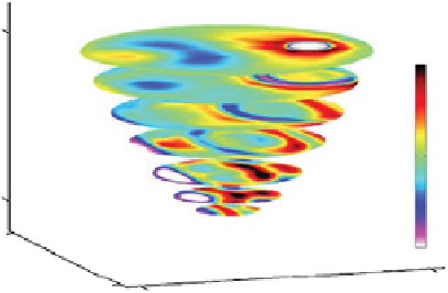
Figure 10.13.
Tomographic reconstruction of internal wave-
field inside a parabolic domain computed from many views
of image displacements such as those in Figure 10.12. Repro-
duced from Figure 4a of
Hazewinkel et al.
[2011].
ρ
on the right-hand side of (10.15), it is efficient
to solve iteratively using the biconjugate gradient method
[
Golub and van Loan
, 1996].
This approach was tested against idealized disturbances
by
Decamp et al.
[2008], who showed that a polar grid is
best used provided the number of sectors is not a multiple
of the number of perspectives. Even with just six per-
spectives, a cosine-times-Gaussian disturbance was well
reproduced on a polar grid with 33 sectors and 40 rings.
Applying this method to internal wave fields generated
in the laboratory has proved challenging in part because
of the requirement to have multiple perspectives. In the
work of
Hazewinkel et al.
[2011], the tank had curved
localized disturbances, the latter approach was found to
be more effective.
The forward problem can thus be written as a coupled
set of 2
n
equations in
N
unknowns. This is cast in matrix
form analogous to equation (10.12):
→
−→
x
T
,
−→
z
T
T
≡
=
G
ρ
,
(10.14)
in which the differentiation operators acting on elements
of
ρ
to give
∇
ρ
are buried inside the components of
G
,