Geoscience Reference
In-Depth Information
displacements at a fixed time and at a fixed height, so
that
z(x)
is taken to be a function only of the along-
tank distance
x
. We seek the corresponding value of
N
2
(r)
, which is assumed to be axisymmetric, varying
with radius
r
.
The inversion problem begins with representing the
along-tank direction by
n
+ 1 discrete points
x
i
=
idx
for
i
=0,
...
,
n
and by discretizing the radial disturbances
by concentric rings of outer radius
r
j
=
(j
+1
/
2
) dr
.So
that the inversion problem is well posed, we take
dr
N
1
2
/
N
0
2
= 0
2
z
T
0
0.5
1
1
L
0
2
N
0
2
N
0
30
60
90
N
1
2
dx
and we set
j
=0,
...
,
n
, in which
j
= 0 signifies the inner-
most circle. The correspondence of the
x
and
r
coordinate
systems is shown in Figure 10.10.
We assume that
N
2
is constant within each annulus in
the central circle. And so we denote
(N
2
)
0
=
N
2
for
0
≡
= cos
-1
(
N
0
) = tan
-1
(
θ
/
∣
k
z
/
k
x
∣
)
ω
N
1
2
/
N
0
2
= 0.25
2
z
r < dr/
2,
(N
2
)
1
=
N
2
for
dr/
2
≤
≤
r <
3
dr/
2,
1
L
(N
2
)
2
=
N
2
for 3
dr/
2
r <
5
dr/
2, etc. Outside the
outermost ring we assume the ambient is undisturbed so
that
N
2
=0.
We now consider the path of light passing in the
y
direc-
tion from the far side of the tank through the disturbance
field to the side of the tank nearest the camera (i.e., from
top to bottom of the schematic in Figure 10.10).
Given values of
N
2
in each ring, we integrate equa-
tions (10.2) and (10.5), summing the discretized equa-
tions to determine the vertical position of light,
z(y)
,
as it crosses each annulus. Doing so requires computing
in advance the distance
dy
ij
that light from location
x
i
crosses the
j
th annulus (with the zeroth “annulus” being
the central circle). Although they could be computed ana-
lytically, these geometric distances are straightforwardly
determined by a numerical algorithm.
The result of the forward problem is a matrix set of
equations,
≤
0
2
N
0
2
N
N
1
2
N
1
2
/
N
0
2
= 4
2
z
1
L
0
2
N
1
2
N
0
30
60
90
N
0
2
θ = cos
-1
(
ω
/
N
0
) = tan
-1
(∣
k
z
/
k
x
∣)
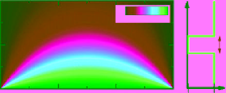
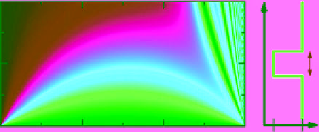
Figure 10.8.
Predicted transmission coefficient for monochro-
matic internal waves of frequency
ω
and horizontal wave num-
ber
k
x
incident upon a region of depth
L
where the ambient
buoyancy frequency is
N
1
instead of
N
0
. Adapted from Figure
1of
Sutherland and Yewchuk
[2004].
−→
z
=
G
−−→
N
2
, (10.12)
in which
−→
z
is the transpose of
(z(
0
)
,
z(x
1
)
,
...
,
z(x
n
))
,
−−→
N
2
is the transpose of
((N
2
)
0
,
(N
2
)
1
,
...
,
(N
2
)
n
)
,and
G
is a square matrix composed of the
distances
dy
ij
and coefficient
γ
defined by (10.6).
Inverting
G
, we can then determine the disturbance field
knowing vertical displacements along a horizontal line:
−−→
through fluid with known varying density (hence with
known varying refractive index). The challenge is to invert
this formula to find the change in stratification for given
observed displacements.
For axisymmetric disturbances about a vertical axis,
the procedure amounts to inverting a square matrix to
determine
N
2
=
G
−
1
−→
z
.
(10.13)
If the image is placed well behind the tank, the compo-
nents of
G
are somewhat more complicated because one
must consider the angle at which light enters the tank from
the image as well as the vertical displacement of light. The
extra terms may be added to components of
G
, akin to
the inclusion of the second term in equation (10.10) for
the spanwise-uniform problem [
Onu et al.
, 2003].
Note that computing
N
2
(r)
need only be done using
image displacements rightward of the center of the dis-
turbance. Independently, one can compute
N
2
(r)
using
ρ
from observed displacements of an image.
For fully three-dimensional disturbances, tomographic
inversion techniques are needed to reconstruct
∇
ρ
from
displacements observed from multiple perspectives.
∇
10.4.1. Axisymmetric Synthetic Schlieren
We consider the simplest case of reconstructing
N
2
from observed vertical displacements of an image,
z
[
Onu et al.
, 2003]. First we consider the vertical