Geoscience Reference
In-Depth Information
computed. Theory was found to be consistent with the
experiments, but there was great sensitivity of the pre-
dicted transmission coefficient to the details of the strati-
fication. For example, referring to Figure 10.8b with
ω
2
Δ
N
-0.01
-0.005
0.005
0.01
0.8
N
, one sees that the transmission coefficient increases
rapidly from 0.4 to 1 as
k
x
L
increases from 0.7 to 1. And
so, uncertainty in the measurement of
k
x
greatly increases
the uncertainty in the predicted transmission. Likewise,
with smooth
N
2
profiles, the predicted transmission coef-
ficient sensitively depends upon the smoothness of
N
,
particularly if the incident wave frequency is close to the
minimum value of
N
[
Gregory and Sutherland
, 2010]. For
those intending to use theory to predict internal wave
transmission, these experiments emphasize the impor-
tance of performing an error analysis for both incident
internal wave properties and the structure of the ambient.
20
10
10
20
30
x
(cm)
40
50
60
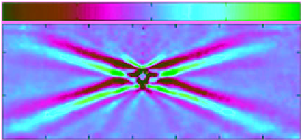
Figure 10.6.
Change in the background squared buoyancy fre-
quency (
N
2
) due to internal waves generated by an oscillating
cylinder, as measured by quantitative synthetic schlieren. The
left image shows a snapshot of the
N
2
field; the right image
shows the amplitude envelope of the wave beams. Reproduced
from Figure 2 of
Mercier et al.
[2008].
10.4. NON-SPANWISE-UNIFORM
DISTURBANCES
The transmission of a small-amplitude wavepacket
through arbitrary stratification and background flow
can be computed through the solution of the Taylor-
Goldstein equation [
Nault and Sutherland
, 2007, 2008].
These results were compared with laboratory experiments
of internal waves incident upon a pycnocline [
Mathur
and Peacock
, 2009] and of internal wave beams incident
upon a weakly stratified layer [
Gregory and Sutherland
,
2010]. Using the Hilbert transform method, the incident,
reflected, and transmitted waves could be distinguished
and so transmission and reflection coefficients could be
The quantitative uses of synthetic schlieren described
above assumed that any disturbances in the stratified fluid
were uniform across the width of the tank. With this
assumption, it was straightforward to relate displacements
of images to changes in stratification through equation
(10.10). It was likewise trivial to invert this equation and so
infer changes in the stratification knowing the measured
displacements, as in equation (10.11).
If disturbances are not spanwise uniform, one can
still use Snell's law to write down expressions for the
apparent displacement of an image due to light passing
k
x
<0 and
k
z
<0
k
x
>0 and
k
z
<0
20
20
10
10
10
20
30
x
(cm)
40
50
60
10
20
30
x
(cm)
40
50
60
2
Δ
N
-0.01
-0.005
0
0.005
0.01
k
x
<0 and
k
z
>0
k
x
>0 and
k
z
>0
20
20
10
10
10
20
30
x
(cm)
40
50
60
10
20
30
x
(cm)
40
50
60
Figure 10.7.
The four arms of the cross shown in Figure 10.6 determined by Fourier implementation of the Hilbert transform.
Reproduced from Figure 3 of
Mercier et al.
[2008].