Geoscience Reference
In-Depth Information
of the QBO. The detailed study of the parametric and
numerical sensitivities reveal the dominant role of wave-
wave and wave-mean flow interactions in the laboratory
flow, with critical layer absorption and viscous dissipation
chronologically secondary to instabilities from nonlinear
flow interactions [
Wedi and Smolarkiewicz
, 2006]. These
findings elevate the importance of the laboratory setup for
its fundamental similarity to the atmosphere, where such
instabilities are observed to occur.
9.2.2.1. Numerical Model.
The Boussinesq equations
of motion, an accurate approximation for salty water
[
Gill
, 1982], for a nonrotating, density-stratified, viscous
fluid are cast in a time-dependent curvilinear framework
[
PrusaandSmolarkiewicz
, 2003;
SmolarkiewiczandPrusa
,
2005]:
∂
ρ
∗
v
s
k
∂x
k
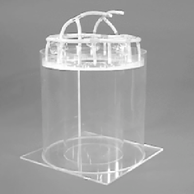
Figure 9.2.
Cylindrical annulus used for the QBO experiments
conducted at the University of Kyoto as part of the GFD-Dennou
Club. Used with permission,
Sakai
[1997] and
Otobe et al.
[1998]. The oscillating membrane can be seen at the top of
the annulus, while in the original experiment of Plumb and
McEwan the membrane was mounted at the bottom.
=0,
d
v
j
dt
=
∂π
∂x
k
−
g
ρ
−
G
j
ρ
0
δ
3
j
+
j
+
j
,
C
F
dρ
dt
=
v
s
k
∂ρ
e
−
∂x
k
+
F
ρ
.
(9.2)
by
Otobe et al.
[1998] is equivalent to the original Plumb
and McEwan experiment, whereas the experimental setup
described by
Sakai
[1997] used an approximately twice
larger domain (2
L
x
,2
L
y
). Their laboratory experiments
and their detailed descriptions of the experiment [cf.
Sakai
, 1997] give interesting insights into the sensitivity
and the difficulties encountered when trying to exactly
reproduce the oscillation period obtained by Plumb and
McEwan. For example, the stratification degraded in the
near-membrane layers, influencing the mean-flow oscil-
lation period. Equally, the tank size and the associated
wavelengths of the forcing have a substantial influence on
the oscillation period [
WediandSmolarkiewicz
, 2006]. The
laboratory experiments at the University of Kyoto show a
range of observed mean-flow oscillation periods of 45-
120 min [
Otobe et al.
, 1998], with several at approximately
1 h. Nevertheless, all these results show that the emerging
zonal mean zonal flow oscillation period is always much
longer than the inverse of the frequency of the forcing
waves.
Here,
ρ
∗
:=
ρ
0
G
, with
G
denoting the Jacobian of
the transformati
o
n
b
et
w
ee
n
physical
(t
,
x
,
y
,
z)
and
computational
(t
,
x
,
y
,
z)
space. Indices
j
,
k
=1,2,3
correspond to the
x
,
y
,
z
components, respectively; sum-
mation is implied by repeated in
d
ices unl
e
ss
st
ated
ot
h-
erwise. The total derivative is
d/dt
=
∂
∂t
+
v
∗
j
(∂
∂x
j
)
,
j
:=
x
j
denotes the contravariant velocity. The
solenoidal veloci
ty
, satisf
yi
ng th
e
mass continuity equa-
tion in (9.2), is
v
s
j
where
v
∗
j
∂x
j
/∂t
.
The components
of physical velocity
v
j
are related via
v
s
k
=
G
j
v
j
,where
G
j
=
(∂x
k
/∂x
j
)
are transformation coefficients;
ρ
and
π
denote density and normalized pressure perturbations,
respectively, with respect to the static ambient state char-
acterized by the linearly stratified profile
ρ
e
=
ρ
0
(
1
:=
v
∗
−
−
(N
2
/g)z)
,
g
symbolizes the gravitational acceleration,
ρ
0
is a constant reference density, and
δ
3
j
is the Kronecker
delta. The change of density due to the diffusivity of salt
in water,
ρ
, and the momentum dissipa-
F
ρ
∼∇·
κ
∇
v
T
)
, are detailed in the work of
Smolarkiewicz and Prusa
[2005]. Here, we specify a kine-
matic viscosity
ν
= 1.004
tion,
F
∼∇·
ν(
∇
v
+
∇
9.2.2. DNS of the Laboratory Analogue of the QBO
10
−
6
m
2
/
s and a diffusivity
×
10
−
9
m
2
/
s
)
. The Coriolis force
of salt in water
κ(
=1.5
×
Incorporating the rapidly undulating boundaries of the
laboratory experiment into the numerical algorithm via
time-dependent curvilinear coordinates allows to repro-
duce the experimental setup while minimizing numerical
uncertainties.
Wedi and Smolarkiewicz
[2006] presented
results of the first DNS of the phenomena that lead to
the zonal mean-flow reversal in the laboratory analogue
j
terms
0.
The generalized Gal-Chen coo
r
dinat
e
transfor
m
ation
assumes identity transformations
t
=
t
,
x
=
x
,and
y
=
y
,
but
C
≡
z
s
(x
,
y
,
t)
H(x
,
y
,
t)
z
−
z
=
H
0
z
s
(x
,
y
,
t)
,
(9.3)
−