Geoscience Reference
In-Depth Information
(a)
(b)
10
3
10
3
10
2
10
2
10
1
10
1
10
0
10
0
10
0
10
0
10
1
10
2
10
3
10
1
10
2
10
3
L
b
(cm)
L
visc
(cm)
(c)
(d)
10
2
10
2
10
1
10
1
10
0
10
0
10
-1
10
-1
10
-1
10
-1
10
0
10
1
10
2
10
0
10
1
10
2
L
0
(cm)
L
d
(cm)
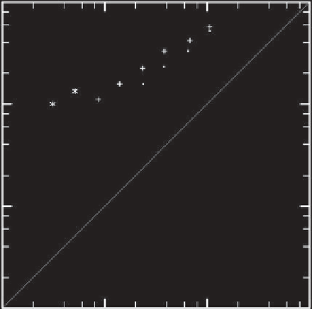
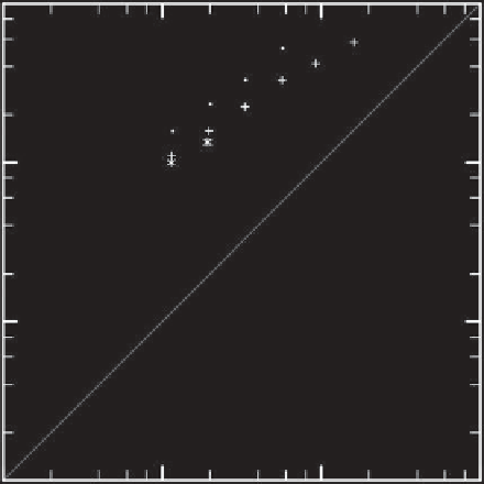
Figure 8.10.
Horizontal scale
L
m
of minimum small-scale buoyancy flux plotted against (a) the buoyancy scale
L
b
, (b) the viscous
scale
L
visc
, (c) the Ozmidov scale
L
O
, and (d) the Kolmogorov scale
L
d
. Symbols denote Re
b
≈
2(
·
), 0.6 (
+
), and 0.2 (
∗
) (simulation
sets A, B, and C).
8.4. DISCUSSION AND CONCLUSIONS
simulations is predominantly downscale, and there is
no evidence of
Lilly's
[1983] hypothesized inverse cas-
cade. Nevertheless, the layerwise structure that he antic-
ipated is clearly visible. The layer thickness scales like the
viscous scale
L
visc
, but for laboratory parameters with
Re
b
∼
The stratified turbulence simulated in these numeri-
cal experiments is surprisingly reminiscent of the pic-
ture painted by
Lilly
[1983], despite the significant
advances in understanding that have occurred over the
last three decades. Of course, the energy transfer in these
O(
1
)
, the viscous scale is very close to the buoy-
ancy scale
L
b
. As a result, the layers in these simulations,