Geoscience Reference
In-Depth Information
(a)
(b)
10
0
10
0
10
-2
10
-2
10
-4
10
-4
10
-6
10
-6
2.6
0.63
0.16
2.3
0.63
0.17
10
-8
10
-8
10
-10
10
-10
10
0
10
0
10
1
10
2
10
3
10
1
10
2
10
3
k
h
/
∆
k
k
h
/
∆
k
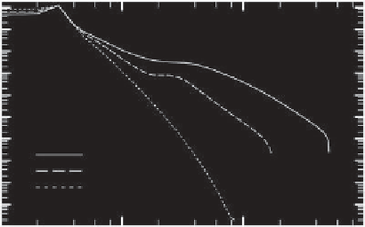
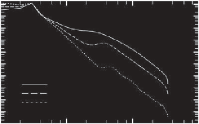
Figure 8.2.
Horizontal wave number spectra of kinetic energy in simulations with (a) fixed
N
= 0.566 s
−1
and different
ν
(and
hence different Re and Re
b
, i.e., runs A6, B4, and C2), and (b) fixed
ν
= 0.0625 cm
2
/s and different
N
(and hence different Fr
h
and Re
b
, i.e., runs A5, B5, and C5). Dash patters denote different Re
b
.
the spectrum exhibits a short power law range downscale
of the forcing with a slope of around -3, followed by a
broad spectral bump at larger
k
h
. As the Reynolds number
(and hence Re
b
) decreases, the spectrum steepens and the
bump is reduced. Similar behavior is displayed in Figure
8.2b, which shows spectra from three simulations with the
same viscosity and different stratifications. The spectra
steepen as the Froude number (and hence Re
b
) decreases,
while the spectral bump shrinks and moves to higher
k
h
.
These changes to the kinetic energy spectrum with Fr
h
and Re can be partially accounted for by a dependence
on Re
b
alone [as in
Brethouwer et al.
, 2007]. Spectra from
all simulations are plotted Figure 8.3, where they are
arranged into groups of approximately equal values of
Re
b
≈
spectra obtained with the lowest Reynolds numbers have
only a short power law range between the forcing and dis-
sipation wave numbers. However, a spectral bump eventu-
ally emerges in each case as Re increases and Fr
h
decreases.
As Re
b
decreases, higher values of Re (and hence smaller
Fr
h
) are required for a spectral bump to appear: For
Re
b
≈
0.2, only the two highest-Re cases exhibit a bump
downscale of the steep
5 spectrum. The position of the
bump appears to move to larger
k
h
as Re increases and
Fr
h
decreases, but its shape is quite variable; in general,
it is broader for large Re
b
, and it narrows (or disappears
entirely) as Re
b
decreases. These findings are reminiscent
of the buoyancy-scale bumps described by
Waite
[2011],
which were located at
k
h
around the buoyancy wave num-
ber
k
b
≡
−
2
π/L
b
≡
2, 0.6, 0.2. The forcing and power law portions of
the spectra collapse fairly well at constant Re
b
,atleast
for
k
h
not too large. The spectral slopes of the power law
range are plotted in Figure 8.4 (slopes are computed with
a least squares fit over 4
N/U
. The possible relationship between
the spectral bumps in Figure 8.3 and the buoyancy scale
is investigated further below.
10; note that for the
lowest Re simulations in Figure 8.3a, there is no clear dis-
tinction between the power law range and spectral bump).
The changes in slope obtained at constant Re
b
are for the
most part much smaller than changes at constant Fr
h
or
Re. All spectra are steeper than
≤
k
h
/k
≤
8.3.3. Energy Budget
The spectral budget of kinetic and potential energy is
governed by the equations
∂
∂t
E
K
(k
h
)
=
T
K
(k
h
)
+
B(k
h
)
5
−
D
K
(k
h
)
+
F(k
h
)
, (8.26)
3
, which as discussed in
Section 8.2.3 is to be expected at these values of Re
b
.Over-
all, smaller Re
b
yield steeper spectra: Slopes are around
−
−
∂
∂t
E
P
(k
h
)
=
T
P
(k
h
)
−
−
B(k
h
)
D
P
(k
h
)
.
(8.27)
2, 0.6, 0.2. The collapse is
very good for smaller Re
b
, where the slopes vary by less
than 10% at constant Re
b
. A greater spread in slopes is
found for Re
b
≈
3,
−
4, and
−
5forRe
b
≈
The terms
T
K
(k
h
)
and
T
P
(k
h
)
are the transfer spectra of
kinetic and potential energy, which represent conserva-
tive exchanges of energy between different wave numbers
by nonlinear interactions. The
B(k)
term is the buoyancy
flux, which is given by the cross spectrum of vertical
velocity and buoyancy; it describes the wave number local
conversion of potential to kinetic energy, and so it appears
in both equations (8.26) and (8.27) with opposite signs.
The
F(k
h
)
term denotes injection of kinetic energy by
2: In these simulations, there is a clear
steepening from around
3asFr
h
decreases and Re
increases, even though Re
b
is approximately constant. The
slopes appear to have not quite converged in this case and
may steepen below
−
2to
−
3 for even smaller Fr
h
and larger Re.
At larger wave numbers the collapse of the spectra in
Figure 8.3 is not particularly good. For each Re
b
,the
−