Geoscience Reference
In-Depth Information
(a)
(b)
R
low
P
up
R
low
0
0
-0.2
-0.2
F
F
-0.4
-0.4
I
-0.6
-0.6
R
up
-0.8
R
up
-0.8
0.06
RR
RF
RF
0.06
0.04
0.02
RP
1
0.02
0.01
0
0
0
5
10
15
20
25
0
5
10
15
20
25
k
k
(c)
R
low
0
-0.2
F
P
up
-0.4
I
R
up
-0.6
-0.8
0.02
RF
RP
n
0.01
0
0
5
10
15
20
25
k
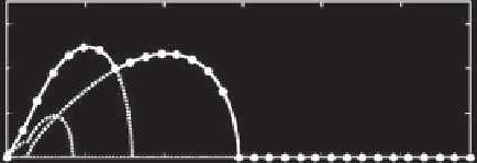
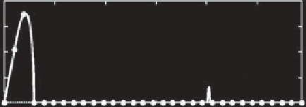
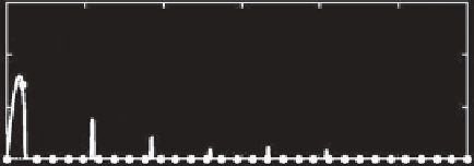
Figure 6.10.
Dispersion diagram (upper panels) and growth rate (lower panels) of the eigenmodes of the outcropping configuration
for (a) Ro = 0.02, (b) Ro = 0.2, and
(c)
Ro = 0.6 with
δ
H
= 0.1. Thick gray lines on the upper panel correspond to the unstable
modes.
in the sense that they behave like Rossby modes as long as
the wave number is small and like gravity modes when the
wave number becomes large. Note that
HayashiandYoung
[1987] and other authors refer to these modes as Kelvin
waves, as they propagate along the (internal) boundary.
More generally, the frontal mode can be interpreted as a
vortical mode, as in the work of
Meacham and Stephens
[2001],
Gula and Zeitlin
[2010], and
Gula et al.
[2010], in
a sense of a wave that exists due to the PV gradient at
the outcropping point, because this point may be inter-
preted as a point connecting the finite-depth layer with
a layer of infinitesimal thickness [
Boss et al.
, 1996]. We
use the denomination “frontal” for such modes in what
follows.
Figure 6.10 shows the dispersion diagram and cor-
responding growth rates of the eigenmodes of the
outcropping coastal flow with a depth ratio
δ
H
=
H
1
(r
1
)/
[
H
1
(r
1
)
+
H
2
(r
1
)
]
= 0.1 and a density ratio
δ
s
=
ρ
1
/ρ
2
=
0.99 as a function of
k
for increasing values of vertical
shear: Ro = 0.02, Ro = 0.2, and Ro = 0.6.
For low Rossby and Burger numbers (Figure 6.10a),
Rossby modes in the lower layer with
c
≈
U
2
=0 can