Geoscience Reference
In-Depth Information
(c)
1
1
1
0.8
0.6
0.4
0.8
0.6
0.4
0.8
0.6
0.4
0.2
0
-0.2
-0.4
0.2
0
-0.2
-0.4
0.2
0
-0.2
-0.4
-0.6
-0.8
-1
-0.6
-0.8
-1
-0.6
-0.8
-1
-1 -0.8 -0.6 -0.4 -0.2
0
0.2
0.4
0.6
0.8
1
-1 -0.8 -0.6 -0.4 -0.2
0
0.2
0.4
0.6
0.8
1
-1 -0.8 -0.6 -0.4 -0.2
0
0.2
0.4
0.6
0.8
1
(d)
0.2
0.2
0.2
0.15
0.15
0.15
0.1
0.1
0.1
0.05
0.05
0.05
0
0
0
-0.05
-0.05
-0.05
-0.1
-0.1
-0.1
-0.15
-0.15
-0.15
-0.2
-0.2
-0.2
-0.2 -0.15
-1
-0.05
0
0.05
0.1
0.15
0.2
-0.2 -0.15
-1
-0.05
0
0.05
0.1
0.15
0.2
-0.2 -0.15
-1
-0.05
0
0.05
0.1
0.15
0.2
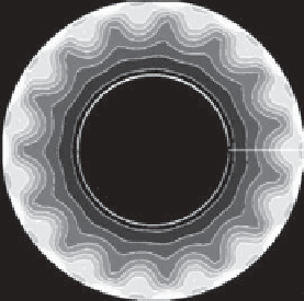
Figure 6.8 Continued.
(c) the unstable RP mode at
k
=15(
kR
d
= 28, see Figure 6.6), and (d) the unstable KK mode at
k
=10
(
kR
d
= 95, see Figure 6.7). The full lines correspond to positive and the dotted lines to negative values. (a) Both fields are typical
of a Rossby mode. (b) The field in the upper layer is typical of a Rossby mode while the field in the lower layer is typical of a
Kelvin mode. (c) The field in the upper layer is typical of a Rossby mode while the field in the lower layer is typical of a Poincaré
mode. (d) Both fields are typical of a Kelvin mode.
section. So we consider now the situation where the inter-
face between the layers joins the free surface forming a
surface front, as shown in Figure 6.9. This is an idealized
configuration of a buoyancy-driven coastal current in a
circular basin. In the classical experiments by
Grifithsand
Linden
[1982], a volume of lighter salty water of density
ρ
1
flows above a denser water of density
ρ
2
and is con-
fined between the surface front and the internal cylinder.
In the work of
Thivolle-Cazat and Sommeria
[2004] and
Pennel et al.
[2012], the lighter fluid flows along the exter-
nal cylinder. In the following we consider an upper layer
of lighter fluid of density
ρ
1
with a free surface terminat-
ing at a point
r
=
r
0
=
r
1
+
L
with mean velocity
U
1
(r)
and a lower layer of density
ρ
2
>ρ
1
with a mean velocity
U
2
(r)
.
We work with the two-layer shallow-water equations in
the cylindrical geometry, as in the previous section, and
perform a cylindrical equivalent of the stability analy-
sis of
Gula and Zeitlin
[2010] and
Gula et al.
[2010] for
coastal currents. Another difference with the previous
section is that we now consider a free surface instead of
a rigid lid for the comparison with experiments. In this
section the slope of the bottom,
γ
, is set to be zero, its
influence to be studied in the next section.
By introducing the time scale 1
/f
, the horizontal scale
L
, which is the unperturbed width of the density current,
the vertical scale
H
0
=
H
1
(r
1
)
, and the velocity scale
fL
,
we use nondimensional variables from now on without
changing notation. Note that with this scaling the charac-
teristic value of the velocity gives the Rossby number. By
linearizing about a steady state in cyclogeostrophic equi-
librium, we obtain nondimensional equations identical to
equations (6.2), where the pressure perturbations in the
layers
π
j
are now related through the layers' heights
h
j
via
the hydrostatic relations as follows:
π
j
=
Bu
(δ
j
−
s
h
1
+
h
2
)
.
∇
2
s
∇
(6.9)