Geoscience Reference
In-Depth Information
(a)
(b)
1
10
-0.02
0.9
9
0.8
-0.04
8
0.7
7
-0.06
0.6
6
-0.08
0.5
5
n
= 2
0.4
-0.1
4
0.3
1
3
-0.12
0.2
0
2
0.1
-0.14
0
0
1
20
40
60
5
10
15
20
25
30
35
40
45
50
k R
b
m
+1
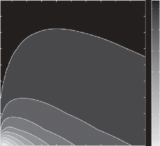
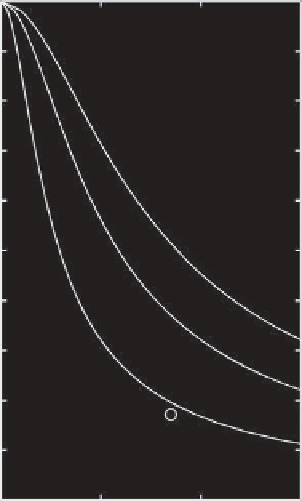
Figure 5.2.
Dispersion relations for (a) inertial waves and (b) Rossby waves. The frequencies of inertial wave modes
n
=0,1,2
are calculated by numerically solving (5.20). The wave vector
k
is nondimensionalized by the barotropic radius of deformation
R
b
. The frequencies of the Rossby waves are calculated from (5.26) for different azimuthal,
m
, and radial,
n
, wave numbers. The
dimensional parameters are
γ
=1.2
10
−3
s
−1
cm
−2
,
R
b
= 21.6 cm,
R
=55cm,and
f
0
=4.58s
−1
. The gray scale shows the
×
dimensionless frequency
ω/f
0
.
Note that the value of the product
γ
n
H
0
should lie
between
(
1+
n)π/
2and
(
1+
n)π
. The dispersion relation
(5.20) is shown in Figure 5.2 a for modes
n
=0,1,2.
Once the vertical structure is resolved, we can eas-
ily write the velocity components in terms of surface
elevation:
Inertial waves are nongeostrophic and nonhydro-
static motions. Within a context of modes propagating
horizontally in the fluid of constant depth, these waves are
described by equations 5.20-5.22. However, if the depth
of the layer is not constant, the modal description can
be used only approximately. Alternatively, without the
assumption of constant depth, inertial waves can be con-
sidered as transverse oscillations with ray paths such that
the angle
θ
between the direction of the wave and the
rotation axes is determined by the frequency of the wave,
θ
= cos
−
1
(ω/f
0
)
(e.g.,
Greenspan
[1968]).
Consider next Rossby waves in a rotating system where
either the Coriolis parameter or the depth of the layer
varies with distance from the pole. While the theory of
Rossby waves on the
β
-plane is very familiar, it is instruc-
tive to consider an alternate version of this theory on the
polar
β
-plane [e.g.,
Rhines
, 2007;
Afanasyev et al.
, 2012]
as follows. The shallow water equation (5.12) can be
completed with a continuity equation [
Gill
, 1982] of
the form
g
iω
∂η
∂η
∂y
cos
γ
n
(z
+
H
0
)
(f
0
−
u
=
−
∂x
+
f
0
,
ω
2
)
cos
γ
n
H
0
v
=
g
f
0
∂η
∂x
−
iω
∂η
∂y
cos
γ
n
(z
+
H
0
)
(f
0
−
,
(5.22)
ω
2
)
cos
γ
n
H
0
giγ
n
η
sin
γ
n
(z
+
H
0
)
ω
cos
γ
n
H
0
−
w
=
.
The relations (5.19) and (5.22) allow us to obtain all of
the characteristics of the inertial wave from its signature
on the surface determined by the surface elevation
η
. Note
that in order to obtain the velocity field the frequency of
the wave has to be measured. This requires a relatively
long set of observations (for the duration of one or more
inertial periods). A Fourier transform can then yield the
frequency.
∂
∂t
η
+
(
V
g
·
∇
)η
+
H
0
(
∇
·
V
a
)
= 0.
(5.23)