Geoscience Reference
In-Depth Information
4.3.3. Axially Rotating Pipe Flow
There have only been a few different experimental
studies of the axially rotating pipe flow. The experimen-
tal challenge is to have a long enough pipe so that both
the rotational effects and the pipe flow itself can become
fully developed. One of the first studies was a stability
experiment by
Nagib et al.
[1971], who used a fairly short
pipe (
L/D
≈
23, where
L
is the length of the pipe and
D
its diameter) so the parabolic profile was not fully devel-
oped; however, the rotation was obtained by the letting
the fluid (water) pass through a porous material inside
the rotating pipe, thereby efficiently bringing the fluid into
rotation. They observed from flow visualization and hot-
film measurements that the transitional Reynolds number
decreased from 2500 to 900 when the swirl rate increased
from 0 to 3. More recently,
Imao et al.
[1992] used a 300
D
long pipe (with water) to study the low stability at low
Reynolds numbers (500-1000) and up to rather high swirl
rates (
S
=0
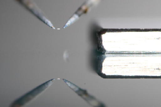
Figure 4.10.
Hot-wire sensor and its reflection close to the
wall for comparative measurement with a 1 mm thick gauge
block in order to determine its position relative to the wall.
The obtainable accuracy is estimated to better than 10
μ
m. The
length of the hot-wire sensor is approximately 0.3 mm. From
Imayama
[2012]. Copyright © Imayama, 2012. Reprinted with
permission.
11). They described details of the instabilities
through both LDV measurements and flow visualizations
and demonstrated that the instability takes the form of
spiral waves.
There have also been a number of experimental inves-
tigations of turbulent pipe flow. One of the first was that
of
White
[1964], followed by
Kikuyama et al.
[1983],
Imao
et al.
[1996], and
Facciolo et al.
[2007]. Only Facciolo et al.
used air as the fluid. One reason why water is preferable to
air is that its lower kinematic viscosity makes it possible to
keep both the Reynolds and swirl numbers high, without
an excessive rotation rate, since
−
based on that calibration method showed satisfactory
consistency.
Another issue related to studies of turbulent boundary
layers over rotating disks is the determination of the skin
friction or, equivalently, the friction velocity (
u
τ
). Since
this quantity is essential for scaling the boundary layer
variables in the turbulent case, a direct measure is nec-
essary and correlations obtained for the well-established
two-dimensional turbulent flat-plate boundary layer can-
not be relied upon. To date, the skin friction has been
obtained through hot-wire measurements in the vis-
cous sublayer close to the disk surface (
z
+
=
zu
τ
/ν
=
z/
V
w
=
S
Re
ν
D
.
Water may also be preferable for studies using LDV or
flow visualization. An advantage of using air is that the
pipe can be open at the end and the flow easily accessed
by probes or LDV.
White
[1964] measured the pressure drop in nonrotat-
ing parts upstream and downstream of the rotating pipe
and found that it, and hence the skin friction, decreased
when rotation was applied.
Kikuyama et al.
[1983] showed
through LDV measurements that the streamwise velocity
profile became less flat and thereby the velocity gradient at
the wall decreased. They also showed that the luid was not
in solid-body rotation but lagged behind, giving a nearly
parabolic profile (illustrated in Figure 4.8). Similar results
were shown by
Imao et al.
[1996] but were also supple-
mented by measurements of five of the shear stresses. The
normal stresses were lower for the cases with rotation.
In the study of
Facciolo et al.
[2007] an airflow facility
was used and a schematic of it is shown in Figure 4.11,
with the major components described in the caption. The
<
6). As an example the thickness of the viscous
sublayer is about 100
μ
m at Re = 800 and a radius of
r
= 400 mm (independent of the fluid), corresponding to
a viscous length scale of about 15
μ
m, emphasizing the
need for very small probes and accurate positioning. So
far, direct measurement of the friction velocity has only
been reported by
Itoh and Hasegawa
[1994], who deter-
mined the skin friction in both the azimuthal and radial
directions, and by
Imayama
[2012]. In the case of hot-wire
measurements of turbulent fluctuations, spatial averaging
of turbulent fluctuations along the sensor may seriously
affect the results (see, e.g.,
Segalini et al.
[2011]). Even a
sensor length of 20
∗
∗
can give reductions of the turbu-
lence intensity of the order of 10% in the near-wall region,
whichmeans that very small sensor lengths need tobeused
in order for the measurements of turbulence quantities
not to be affected by spatial averaging.