Geoscience Reference
In-Depth Information
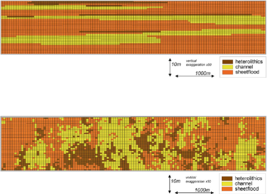
Fig. 2.35
Rock modelling using indicator kriging
Fig. 2.36
Rock modelling using SIS
Models built with SIS should, by definition,
honour the input element proportions from wells,
and each geostatistical realisation will differ
when different random seeds are used. Only
when large ranges or trends are introduced will
an SIS realisation differ from the input well data.
The main limitation with such pixel-based
methods is that it is difficult to build architectures
with well-defined margins and discrete shapes
because the geostatistical algorithms tend to cre-
ate smoothly-varying fields (e.g. Fig.
2.36
).
Pixel-based methods tend to generate models
with limited linear trends, controlled by the prin-
cipal axes of the variogram. Where the rock units
have discrete, well-defined geometries or they
have a range of orientations (e.g. radial patterns),
object-based methods are preferable to SIS.
SIS is useful where the reservoir elements do not
have discrete geometries either because they have
irregular shapes or variable sizes. SIS also gives
good models in reservoirs with many closely-
spaced wells and many well-to-well correlations.
The method is more robust than object modelling
for handling complex well-conditioning cases and
the funnelling effect is avoided. The method also
avoids the bulls-eyes around wells which are com-
mon in Indicator Kriging.
The algorithm can be used to create
correlations by adjusting the variogram range
to be greater than the well spacing. In the
example in Fig.
2.37
, correlated shales (shown
in blue) have been modelled using SIS.
These correlations contain a probabilistic
component, will vary from realisation to
realisation and will not necessarily create
100 % presence of the modelled element between
wells. Depending on the underlying concept,
this may be desirable.