Geoscience Reference
In-Depth Information
Fuller discussions of these methods are found
in, for example, Barker and Thibeau (
1997
),
Ekran and Aasen (
2000
), Pickup et al. (
2005
).
Reservoir simulators generally perform
dynamic
multi-phase flow simulations - that is,
the pressures and saturations are allowed to vary
with position and time in the simulation grid. The
Kyte and Berry (
1975
) upscaling method is the
most well-known dynamic two-phase upscaling
method, but there have been many alternatives
proposed, such as Stone's (
1991
) method and
Todd and Longstaff (
1972
) for miscible gas.
The strength of the dynamic methods is that
they attempt to capture the '
true'
flow behaviour
for a given set of boundary conditions. Their
principle weaknesses are that they can be diffi-
cult and time-consuming to calculate and can be
plagued by numerical errors.
In contrast, the steady-state methods are easier
to calculate and understand and represent ideal
multi-phase flow behaviour. There are three
steady-state end-member assumptions:
•
Viscous limit
(VL): The assumption that the
flow is steady state at a given, constant frac-
tional flow. Capillary pressure is assumed to
be zero.
•
Capillary equilibrium
(CE): The assumption
that the saturations are completely controlled
by capillary pressure. Applied pressure
gradients are assumed to be zero or negligible.
•
Gravity-Capillary equilibrium
(GCE): Similar
to CE, except that in addition the saturations
are also controlled by the effect of gravity on
the fluid density difference. Note that GCE is
similar to the vertical equilibrium (VE)
assumption also applied in reservoir simulation
(Coats et al.
1971
), except that VE assumes
negligible capillary pressure.
The viscous limit assumption is similar to a
steady-state core flood experiment which is
sometimes used in core analysis of multi-phase
flow (referred to as special core analysis, or
SCAL). Here, a known and constant fraction of
oil and water is injected into the sample (let us
say 20 % oil and 80 % water) and the permeabil-
ity for each phase is calculated from the pressure
drop and flow rate for that phase. The procedure
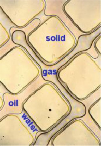
Fig. 4.8
Example micro-model, where fluid distributions
are visualised within an artificial laboratory pore-space
(Statoil
archive
image of micromodel
experiment
conducted at Heriot Watt University)
Another response - the laboratory approach - is
that you need to measure the multiphase flow
behaviour in real rock samples at true reservoir
conditions (pressures and temperatures). In real-
ity, you need both measurements and modelling
to obtain a good appreciation of the “rules”
governing multiphase flow. Our concern here is
to understand how to handle and upscale these
functions within the reservoir model.
4.2.2 Two-Phase Steady-State
Upscaling Methods
Multiphase flow upscaling, involves the process
of calculating the large-scale multiphase flows
given a known distribution of the small-scale
petrophysical properties and flow functions.
There are many methods for doing this, but it is
useful to differentiate two:
1. Dynamic methods
2. Steady-state methods