Geoscience Reference
In-Depth Information
and distribution are known and that they are
statistically stationary (i.e. a global mean).
Ordi-
nary Kriging
is more commonly used because it
assumes slightly weaker constraints, namely that
the mean is unknown but constant (i.e. a local
mean) and that the variogram function is known.
Fuller discussion of the Kriging method can be
found in many textbooks; Jensen et al. (
2000
)
and Leuangthong et al. (
2011
) give very accessi-
ble accounts for non-specialists.
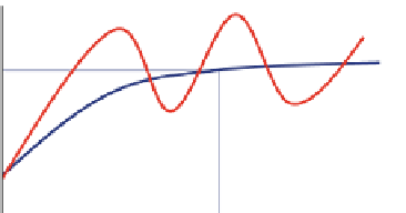
fact close to the variance of the population. The
range (equivalent to the correlation length)
describes the 'separation distance' at which this
occurs. A theoretical semi-variogram has a
smooth function rising up towards the variance
while measured/observed semi-variogram often
has oscillations and complex variations due to,
for example, cyclicity in rock architecture.
The most common functions for the semi-
variogram are spherical, Gaussian and exponen-
tial - each giving a different rate of rise towards
the sill value (ref. Fig.
2.24
). Note that for a
specific situation (second order stationarity) the
semi-variogram is the inverse of the covariance
(de Marsilly
1986
, p. 292). Jensen et al. (
1995
)
and Jensen et al. (
2000
) give a more extensive
discussion on the application of the semi-
variogram to permeability data in the petroleum
reservoirs.
3.4.2 The Variogram
The variogram function describes the expected
spatial variation of a property. In Chap.
2
we
discussed the ability of the variogram to capture
element architecture. Here we employ the same
function as a modelling tool to estimate spatial
property variations within that architecture. We
recall that the semi-variance is half the expected
value of
3.4.3 Gaussian Simulation
the squared differences
in values
separated by h:
Gaussian Simulation covers a number of related
approaches for estimating reservoir properties
away from known points (well observations).
The Sequential Gaussian Simulation (SGS)
method can be summarized by the following
steps (Jensen et al.
2000
):
1. Transform the sampled data to be Gaussian;
2. Assign unconditioned cells
n
o
1
2
EZx
2
ʳ
ðÞ
¼
h
½
ð
þ
h
Þ
Zx
ðÞ
ð
3
:
26
Þ
The semi-variogram (Fig.
3.22
) has several
important features. The lag (h) is the separation
between two points. Two adjacent points will
tend to be similar and have a
(h) of close to
zero. A positive value at zero lag is known as the
nugget. As the lag increases the chance of two
points having a similar value decreases, and at
some distance a sill is reached where the average
difference between two points is large, and in
ʳ
¼
(inter-well)
conditioned cells (wells);
3. Define a random path to visit each cell;
4. For each cell locate a specified number of
conditioning data (the neighbourhood);
5. Perform Kriging in the neighbourhood to
determine the local mean and variance
(using the variogram as a constraint);
6. Draw a random number to sample the Gauss-
ian distribution (from step 5);
7. Add the new simulated value to the “known”
data. Repeat step 4.
Repeating steps 4-7 gives one realisation of a
Gaussian random distribution conditioned to
known points. Repeating step 3 gives a new
realisation. The average of a large number of
realisations will approach the kriged result. In
this way we can use Gaussian simulation to
g
(h)
Sill
Nugget
Range
Lag
Fig. 3.22
Sketch of the semi-variogram (
blue
¼
theoret-
ical function;
red
¼
function through observed data
points)