Geoscience Reference
In-Depth Information
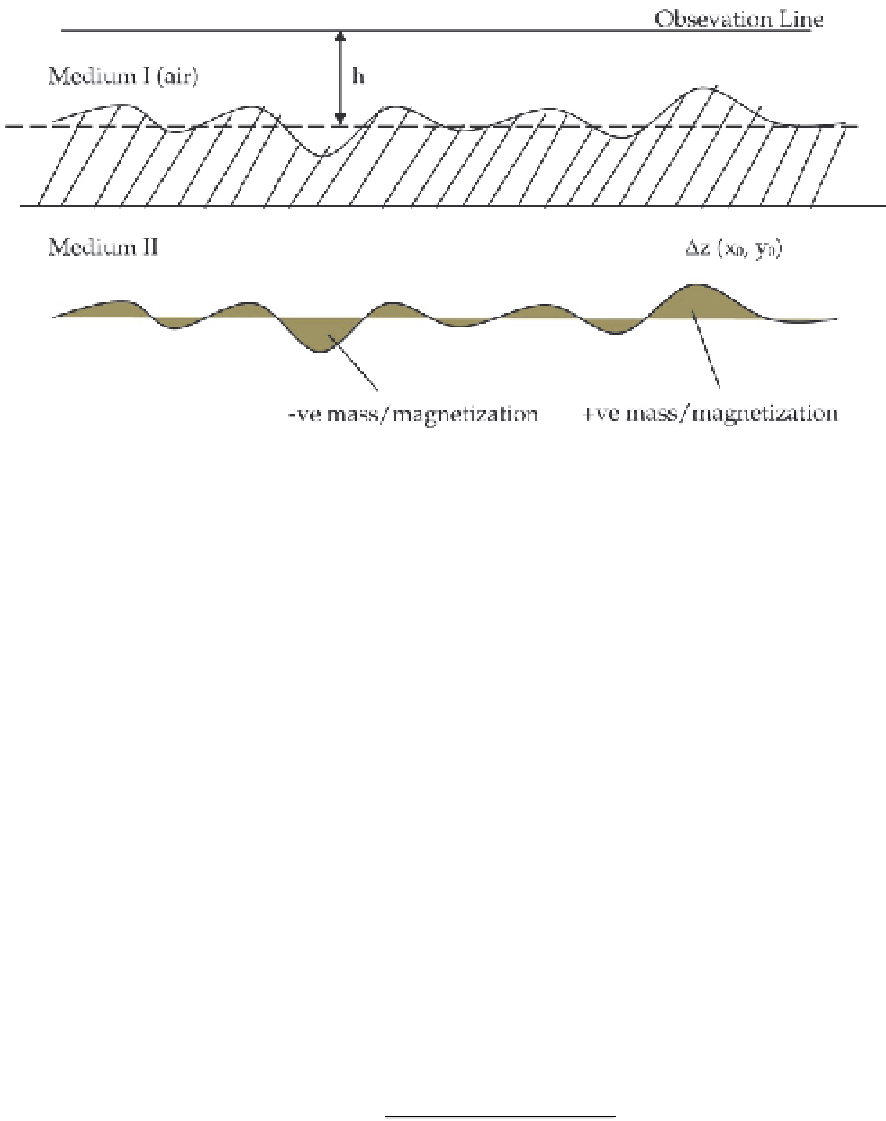
Fig. 2. A homogeneous random interface separating two media of uniform
density/magnetization
(,,)=
∬
dΦ(,)exp(−)exp[(+)]
(30)
The spectral representation of the three components (x, y, z) of the potential field is easily
obtained by differentiating equation (30) with respect to the coordinate axis
(
,,
)
=−
,
(
,,
)
=−
,
and the spectrum of the potential field and its components may also be obtained from
equation (30).
The cross-spectrums between different components can also be computed from the field
equations resulting from the coordinate components obtained from equation (30).
We again look at the random interface (Fig. 2) for the cases of gravity and magnetic fields.
Here we see that the potential field is observed on a plane, h unit above the interface.
Medium I can be replaced with a vacuum (i.e. where density/magnetization = 0) and the
lower medium (Medium II) is characterized by density or magnetization equal to the
difference in density or magnetization of Medium I and Medium II. It is easy to see that the
observed field will consist of two components: a constant part representing the field due to a
semi-finite medium with its upper surface as a horizontal surface, and a random component
representing the field due to the random interface.
For the gravity aspect, the vertical gravity field due to a random interface on the observation
plane may be expressed as (Telford et al., 1990; Roy, 2008)
(
)
[
(
)
(
)
(
)
]
(
,,ℎ
)
=−∬
(31)
Where ∆ρ is density contrast between Medium II and Medium I with the mass element
located at point (x
0
, y
0
, z
0
) and ∆z(x
0
, y
0
) is a homogeneous random function. Equation (31)
can be further expressed using a generalized Fourier transform, ∆Z(u, v) of the random
function, ∆z(x, y) as (Naidu & Mathew, 1998)


Search WWH ::

Custom Search