Next Generation Geological Modeling for Hydrocarbon Reservoir Characterization - Advances in Data, Methods, Models and Their Applications in Geoscience - page 229

2

Ndj

 







obs cal



J  y t   t y t   f ( t )

(8)



j i j j i



j

i  1

obs
j

cal
j

where N dj stands for the number of observed data ( d ) at well j and y and y correspond

to observed and calculated production data, respectively, at well j .

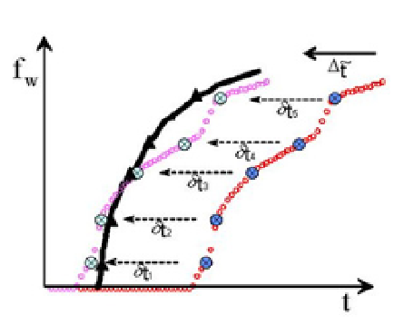
Fig. 10. Illustration of Generalized Travel-Time (GTT) inversion by systematically shifting
the calculated fractional flow curve f w to the observed history (modified from Datta-Gupta
and King, 2007). Red and magenta symbols correspond to the initially-calculated and shifted
curve, respectively, while the black line represents the observed curve.

This is illustrated in Fig. 10, where the calculated fractional flow response 1 is systematically
shifted in small-time increments towards the observed response, every data point in the
fractional-flow curve has the same shift time,

   and the data misfit is
computed for each time increment. The misfit function J directly corresponds to the term
dg(m) , given in Eqs. 5 and 7 that defines the misfit between the observed data and
simulated response. The objective of HM inversion workflow is to minimize the misfit in
production response by reconciling the geological model with observed (measured)
dynamic production data.
The two-step MCMC algorithm (Efendiev et al. 2005) uses an approximate likelihood
calculation to improve on the (low) acceptance rate of the one-step algorithm (Ma et al ,
2008). This approach does not compromise the rigor in traditional MCMC sampling, as it
adequately samples from the posterior distribution and obeys the detailed balance (Maučec et
al., 2007), thus, a sufficient condition for a unique stationary distribution. The main steps of
the streamline-based, two-step MCMC algorithm are depicted in a flowchart in Fig. 11.
A pre-screening based on approximate likelihood calculations eliminates most of the
rejected samples, and the exact MCMC is performed only on the accepted proposals, with
higher acceptance rate. The approximate likelihood calculations are fast and typically
involve a linearized approximation around an already accepted state rather than an
1 In water-injection EOR operations, the fractional flow curve frequently corresponds to water-cut curve
that represents the water breakthrough at the well as a function of well production time.

t t ... t

1 2