Climatic Data - Climate Change: Identification and Projections - page 25

proxies in Figure 2.8 to the following two composite lines: firstly, lean0, for
its proportionality to sun spots, and secondly timv15, which is the most
recent (2014). In this way, we are able to obtain the four reconstructions
given in Figure 2.12, in the graphs on the left.

Usoskin e t be10, c onnected t o timv15 Calib r ation a n d alignment on timv15

1362 1362

1361 1361

Usoskin
Be10
t imv15

1360 1360

1359 1359

0 500 1000 1500 2000 1500 1600 1700 1800 1900 2000

Usoskin et be10, c onnected to lean0 Cali b r ation a nd alig n ment o n lean0

1362 1362

1361 1361

Usoskin
Be10
l ean0

1360 1360

1359 1359

0 500 1000 1500 2000 1500 1600 1700 1800 1900 2000

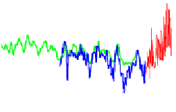
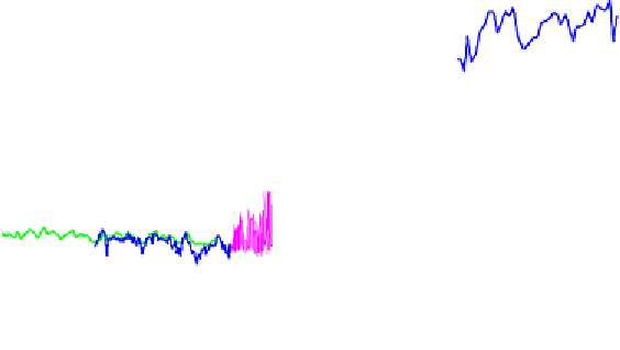
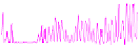
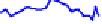
Figure 2.12. Four irradiance reconstructions

In order to carry out the splicing, we determine by least squares, over the
period of overlap, an affine transformation y = ax + b between reference y
(lean0 or timv15 as appropriate) and the series x to be connected.
Subsequently, we apply the relation obtained for the whole series x , and
connect from 1700 onwards. The graphs on the right in Figure 2.12 highlight
the quality of the connection, significantly better for irradiance than they are
for temperatures (see Figure 2.4). Other options could have been considered;
the analysis of principle components, for instance, or possibly using non-
centered PCAs. Fortunately, the quality of the overlap is good enough so that
the technique used only has a minimal impact on the result.

Depending on the option (lean0 or timv15), the amplitude of the
excursions ranges from around one to three. As a result, it is not surprising to
identify solar sensitivity coefficients which have the same ratio, according to
the reconstruction adopted.