Response to forcing: the governing equations and some basic solutions - Introduction to the Physical and Biological Oceanography of Shelf Seas - page 61

3.3.1 The dynamical balance

For a frictionless ocean (t x ¼ t y ¼

@ @ ¼ @ @ ¼

0) in a steady state of motion ( u/ t v/ t 0)

with no external forces acting (F x ¼

F y ¼

0), the linearised momentum equations
(3.13) reduce to a balance between the pressure gradient and the Coriolis force:

0 @ 0 @

1 p 1 p

fu ¼

y ;

fv ¼ ð 3 : 16 Þ

@ @ x

where r 0 is the average density introduced in the last section. These are the equations
of geostrophic flow. Squaring and adding the two relations gives:

! !

2
þ @

2 2

1 @ p p 1 @ p

f 2 u 2 v 2 f 2 C g ¼

ð þ Þ¼ ¼ ð : Þ

3 17

0

@ x @ y

2

@ n

which relates the current speed C g to the magnitude of the pressure gradient @ p/ @ n,i.e.:

0 f @

1 p

C g ¼

n :

ð 3 : 18 Þ

@

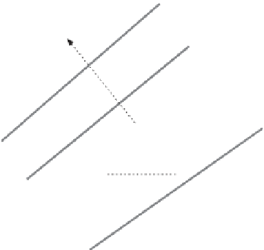
The derivative n here is taken in a direction n normal to the isobars which is the

direction of maximum gradient, illustrated in Fig. 3.4 . In much of the rest of this
discussion we will use n as our general horizontal axis. The direction of the flow is at
an angle c which can be found by dividing the x and y equations (3.16) to give:

@ p/ @

:

v

u ¼ @

p =@ x

tan c ¼ ð 3 : 19 Þ

@ p =@ y

This tells us something very important about the direction of a geostrophic flow.
The direction of an isobar in the horizontal plane ( @ y/ @ x) p is set by the condition that

Figure 3.4 Geometry of isobars
in the horizontal plane.

p 1

C g

v

y

n

p 2

u

p 3

p 4

y

y

x