Waves, turbulent motions and mixing - Introduction to the Physical and Biological Oceanography of Shelf Seas - page 112

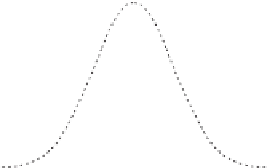
Figure 4.11 Distribution of
1 kg of dye released at x

9

1h

0
into a canal extending in the
x direction. There is no
advection (U ¼ 0) and the
diffusion is Fickian with
an eddy diffusivity of
K ¼ 25 m 2 s 1 . The plot shows
the concentration of dye
(kg m 1 ) at times in hours
after the release.

¼

8

K = 25 m 2 s -1

7

6

5

5h

4

3

2 5 h

2

1

50h

0

-5 -4 -3 -2 -1 0 1 2 3 5

4

x (km)

Suppose that we make a series of dye release experiments corresponding to the
above solutions of the diffusion equation. Because of the random nature of turbu-
lence, each individual release will result in a dye distribution different from the others
and not conforming exactly to the concentration function derived. What is the
relation between these individual realisations of the experiment and the solution of
the differential equations? The answer is that the concentration functions represent
the average of a large ensemble of identical dye experiments and can be thought of as
the probability distribution of dye. So they give us a rather smooth picture of
diffusion which does not include the random nature of individual dye releases.
An alternative method, which better catches the random aspect of turbulence,
relies on a random walk approach. Instead of deriving solutions to the diffusion
equation, we concentrate on the motion of individual 'particles' of dye. To represent
the chaotic movement of particles in turbulent flow, the particles are subjected to a
large number of small random movements.
As an example, consider the 1D dispersion of a large number of particles released
at the origin (x

¼ 0) along the x axis corresponding to the canal diffusion scenario.

At each time step x in the positive or negative x

direction according to the toss of an unbiased coin. After n time steps, the particles
will spread out over a range -n

D t, the particles move a distance D

x with the most likely position being at the
origin. The particles will be distributed along the x axis with a probability given by
the binomial distribution with a mean square deviation after time t

D x to þ n D

¼ n D t given by

2

¼ ð

x Þ

2

2

¼ n ð x Þ t ¼ 2Kt : ð 4 : 44 Þ

t

So the particles disperse from the origin with s increasing as t 1

= 2 and a diffusivity

x) 2 /2

K ¼ ( D D t. For a large enough number of steps n, the binomial distribution