Geoscience Reference
In-Depth Information
V
c
x
0
Fig. 9.5
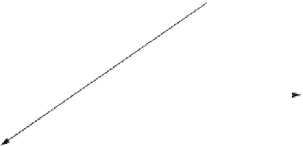
A model of electric charge distribution near the tip and sides of thin tension crack growing
in a sample (Surkov
1986
)
Z
t
exp
t
0
=
r
2
n
r
;t
0
dt
0
:
D
qD exp .
t=/
(9.34)
0
The point defects/dislocations distribution in the plastic zone is assumed to be quasi-
stationary. This implies that the defect number density is a function of variables
D
.x
V
c
t/=
k
and
z
, where
k
is the characteristic length of the plastic zone.
To be specific, consider the following approximation
n
D
n
m
.1
exp .// exp .
j
y
j
=
?
/.
/;
D
.x
v
c
t/=
k
; (9.35)
where n
m
is maximum of the defect number density,
?
is characteristic transverse
size of the plastic zone, and is the step-function. This implies that n
D
0 as >0;
that is, in front of the crack. In the region <0the function n decreases with the
increase of distance from the crack tip.
Consider first the extreme case when the characteristic length of the charge
relaxation due to conductivity is much greater than the typical scales of the plastic
zones, that is, l
r
D
V
c
k
;
?
and
t. Solution of the problem shows
that the electric charges predominantly pile up around the crack tip in the inner
region of plastic zone in such a way that the charge per unit length of the crack
front is Q
D
2qDn
m
t
?
=
k
. Additionally, the charges are distributed along the
crack sides in the DEL. This surface layer with width of the order of
?
has the
total charge
Q: Both these charges vary proportional to time. In the inverse case
when t
, the charge per unit length of the crack front becomes approximately
constant: Q
D
2qDn
m
?
=
k
. The schematic charge distribution for the case of
q>0is displayed in Fig.
9.5
, and in this case the crack tip carries the positive
charge Q. The mobile positive defects diffuse from the crack surface into the sample
thereby producing the shortage of positive charges in the surface layer.


Search WWH ::

Custom Search