Magnetospheric MHD Resonances and ULF Pulsations - Ultra and Extremely Low Frequency Electromagnetic Fields - page 252

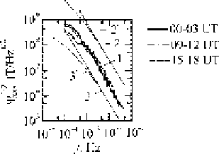
Fig. 6.14 Measured monthly average 3-h power spectra taken from Lanzerotti et al. ( 1990 )
(curve 1) and calculated power spectra of magnetic noise for the nighttime (2) and daytime
(3) ionospheric parameters. The numerical calculations from improved equation ( 6.107 ) are shown
with lines 2 0 and 3 0

The parameters appearing in empirical Eq. ( 6.103 ) is chosen as follows: K D 1 and
m D 2. When Eq. ( 6.105 ) is compared with the evidence from ULF measurements
(Lanzerotti et al. 1990 ), it is apparent that the spectral index n D 1 is a best fit value.
A model calculation of the square root of the spectral amplitude with a best fit
value n D 1 and of the power spectrum recorded at Arrival Heights, Antarctica
in June 1986 (Lanzerotti et al. 1990 ) are presented in Fig. 6.14 as a function of
frequency f . The observational data taken from Lanzerotti et al. ( 1990 ) are shown
with line 1 while our model calculations are plotted with line 2 (daytime conditions)
and 3 (nighttime conditions). It is obvious from Fig. 6.14 that the observational
data are sandwiched between the theoretical lines 1 and 2. It should be noted that
there are some uncertainties in the ionospheric current parameters, for example, in
the constant K in Eq. ( 6.104 ).
We recall that 1D distribution of the ionospheric wind-driven currents results in
the 2D spectral amplitude in inverse proportion to the squared frequency, which in
turn leads to a discrepancy between the predicted and measured spectra.
The observational data slightly deviate from the straight line as is seen in the
upper corner of Fig. 6.14 . In this frequency range the correlation radius may be
greater than or equal to the distance between the Earth and the ionosphere. In such
a case the approximate solution given by Eq. ( 6.89 ) should be replaced by the more
accurate solution. To gain better understanding of this behavior of the observational
data, consider the case x D y D c .!/. Substituting Eqs. ( 6.84 ), ( 6.87 )into
Eq. ( 6.81 ) and applying an inverse Bessel transform yields

1

c .!/ exp 4d 2

1 erf 2d
c .!/

:

0 ‚.!/
32

2 1=2 d

‰ .B/

xx .!/ D

c .!/

(6.107)

Given the above parameters and based on Eq. ( 6.107 ), the numerical calculations
are shown in Fig. 6.14 with lines 2 0 and 3 0 . In the low-frequency limit, when
c .!/ 2d, the expression in square bracket tends to unity whence it follows
that ‰ .B/

xx .!/ / ‚.!/ / ! 1 . This means that the spectral index of the power