Geoscience Reference
In-Depth Information
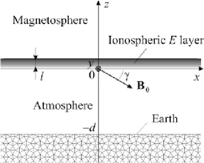
Fig. 6.12
Schematic illustration of a stratified medium model
@
y
ıB
z
@
z
ıB
y
D
0
n
k
E
k
cos
C
J
?
sin
C
J
.
w
x
o
;
(6.61)
@
z
ıB
x
@
x
ıB
z
D
0
n
P
E
y
H
.E
x
sin
C
E
z
cos /
C
J
.
w
y
o
;
(6.62)
@
x
ıB
y
@
y
ıB
x
D
0
n
o
;
k
E
k
sin
C
J
?
cos
C
J
.
w
/
(6.63)
z
where as before
k
denotes the field-aligned plasma conductivity,
H
and
P
are the
Hall and Pedersen conductivities. Here we made use of the following abbreviations:
E
k
D
E
x
cos
E
z
sin ;
(6.64)
J
?
D
P
.E
x
sin
C
E
z
cos /
C
H
E
y
:
(6.65)
The wind-driven current density is given by
J
.
w
x
D
B
0
H
V
?
P
V
y
sin ; J
.
w
z
D
J
.
w
x
cot ;
J
.
w
y
D
B
0
H
V
?
C
P
V
y
;
(6.66)
where V
x
, V
y
and V
z
are the component of the mass velocity of the neutral wind,
and V
?
D
V
x
sin
C
V
z
cos . Notice that the neutral gas dominates below 130 km
in such a way that the charged particles cannot greatly affect the neutral gas
flow. This implies that the mass gas velocity can be considered as a given/forcing
function which affects the electromagnetic fields and conduction currents inside the
conducting E layer of the ionosphere. Furthermore, the parallel plasma conductivity
in this region is much greater than the Hall and Pedersen ones. Assuming that
k
!1
, the parallel electric field
E
k
thus becomes zero, i.e.,
E
z
sin
D
E
x
cos :
(6.67)
Search WWH ::

Custom Search