Geoscience Reference
In-Depth Information
Day
Day
a
b
25
0
F
20
−0.1
F
15
−0.2
10
−0.3
S
5
−0.4
S
0
−0.5
0
0.01
0.02
0.03
0.04
0
0.01
0.02
0.03
0.04
k
, km
−1
k
, km
−1
Night
Night
c
d
25
0
20
F
15
−0.1
F
10
S
5
−0.2
S
0
0
0.01
0.02
0.03
0.04
0
0.01
0.02
0.03
0.04
k
, km
−1
k
, km
−1
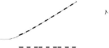
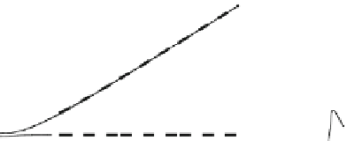
Fig. 5.5
The plots of the real (
a
,
c
) and imaginary (
b
,
d
) parts of the dimensionless frequency x
0
as a function of perpendicular wave number k for the fundamental mode. S and F denote the shear
Alfvén and fast magnetosonic modes, respectively. The
dashed lines
correspond to the approximate
analytical formulae. Taken from Surkov et al. (
2004
)
the results of numerical analysis of Eq. (
5.36
) for the fundamental mode .n
D
1/.
Figure
5.5
a,b show the real and imaginary parts of dimensionless frequency x
0
as
a function of k
?
(in inverse kilometers) for the daytime conditions. A similar plot
for the nighttime conditions is depicted in Fig.
5.5
c,d. The numerical values for the
various magnetospheric, ionospheric, and other parameters are: V
AI
D
500 km/s,
V
AM
D
5
10
3
km/s, L
D
500 km, d
D
100 km, and
g
D
2
10
3
S/m. For
the daytime ionosphere (Fig.
5.5
a,b) the height-integrated conductivities are †
P
D
5 Ohm
1
and †
H
D
7:5 Ohm
1
, respectively, so that Ǜ
P
D
3:14 and Ǜ
H
D
4:71.
The nighttime parameters of the ionosphere are as follows: †
P
D
0:2 Ohm
1
and
†
H
D
0:3 Ohm
1
(Fig.
5.5
c,d), so that Ǜ
P
D
0:126 and Ǜ
H
D
0:188.
The real part of x
0
, which is denoted by , defines the eigenfrequency of the
fundamental mode. As is seen from Fig.
5.5
a,c, the fundamental eigenfrequency
of the shear Alfvén mode, shown with solid lines S, practically does not depend on
k
?
. At the same time, the FMS mode shown in Fig.
5.5
a,c with solid lines F exhibits
approximately linear response to k
?
if k
?
> 0:01 km
1
. As we have noted above,


Search WWH ::

Custom Search