Information Technology Reference
In-Depth Information
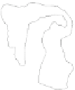
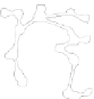
(a) MapSets
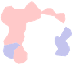
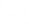
(b) GMap
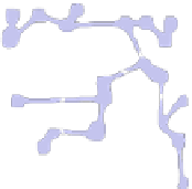
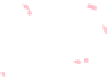
(c) BubbleSets
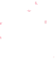
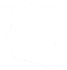
(d) KelpFusion
Fig. 6.
The senator votinggraph (the part of the U.S. west of Mississippi). The vertices are sena-
tors (red republicans and blue democrats) positioned according to their home-cities.
regions grouping together labels and curves in the same cluster. As in GMap, we gen-
erate boundaries by adding dummy points to the current embedding. There are three
types of the dummy points: (a) random points, sufficiently far away from the set of the
input labels, lead to more rounded and thus more realistic region boundaries; (b) ran-
dom points along bounding boxes of the labels help ensure that the labels are drawn
inside the regions; (c) auxiliary points along all the edges constructed on the previous
step, that keep the regions connected. The distance between consecutive points on an
edge is chosen to be less than the distance to any other point of a different color. After
adding the dummy points, we compute the Voronoi diagram of the set of all points and
merge the Voronoi cells that belong to the points of the same color.
TimeComplexity.
Now we discuss the complexity of ouralgorithmonaninput with
n
points and
k
clusters, assuming we can compute distances and intersections between
geometric primitives (points, line-segments, rectangles) in constant time. The sparse
visibility graph can be constructed in
O
(
n
log
n
) time and it contains
O
(
n
) edges [8].
Therefore, computing all pairwise distances takes
O
(
n
2
) time and finding a minimum
spanning tree for one cluster takes
O
(
n
2
+
n
log
n
) time. Summing over all clusters, we
get
O
(
kn
2
). In the iterative force-directed heuristic we compute forces between pairs
of edges, which can take
O
(
n
2
) in the worst case. Hence, the time complexity of the
force-directed heuristic is
O
(
cn
2
),where
c
is the maximumnumber of iterations in the
adjustment (
c
=10in our implementation). The complexity of the edgeaugmentation
step is
O
(
n
3
), as we may add quadratic number of edges in the greedy process. Finally,
computing the boundaries takes
O
(
n
log
n
) time. Therefore, the overall time complexity
is
O
(
kn
2
+
n
3
). More details and actual running times are given in the next section.
5
Experiments
Here we compare ournewalgorithm, MapSets, with the existing approaches for map-
like visualizations: GMap [9], BubbleSets [6], and KelpFusion [15]. A fully functional
implementation of MapSets, GMap, and BubbleSets, together with a complete dataset,
Our first example is the senator votinggraph; see Fig. 6. The vertices in the graph
are the U.S. senators in 2010 positioned according to their home-cities in the U.S. The