Information Technology Reference
In-Depth Information
T
[0]
[1]
[0]
E
E
E
F
F
F
T
[0]
[1]
D
D
D
[0]
G
G
G
[0]
B
B
B
T
T
T
T
[1]
[1]
[1]
[0]
[1]
A
C
A
C
W
2
A
C
T
[0]
[0..2]
[1]
(a)
(b)
(c)
e'
e"
(d)
(e)
(f)
(g)
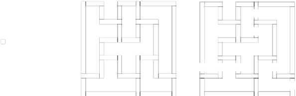
Fig. 3.
(a) An orthogonal drawing
ʓ
D
of the dual graph
D
. (b) The positive instance
F
of HV-
planarity testing built by Step 4. (c) The instance
G
of HV-planarity testing corresponding to the
S
WITCH
F
LOW
N
ETWORK
instance
N
depicted in Fig. 2(a). (d) Tendril
T
1
.Edges
e
and
e
are
the handles of the tendril. (e) Tendril
T
2
. (f) Wiggle
W
1
.(g)Wiggle
W
2
.
−
4
h
and 4
h
, respectively) right angles. Since in any HV-realization of
G
,thesubgraph
of
G
obtained by neglecting tendrils and wiggles is drawn as it is in
F
, and since in
F
each face is balanced in terms of left and right turns, it follows that the HV-realization
chosen for tendrils and wiggles of
G
decides a flow traversing the faces of
G
. By con-
struction, such a flow (divided by 4) gives a feasible flow for
N
.Conversely,suppose
a feasible flow exists for
. By choosing the corresponding HV-realizations for ten-
drils and wiggles, each face is balanced in terms of right and left angles, yielding an
HV-realization for
G
.
N
3
Testing Algorithm for Series-Parallel Graphs
The decomposition of a biconnected graph
G
into its triconnected components is de-
scribed by the
SPQR-tree
data structure, which implicitly represents all planar embed-
dingsof
G
.Weassume familiarity with
SPQR
-trees and related terminology[4].If
the
SPQR
-tree
T
of
G
has no
R
-nodes (corresponding to triconnected components
that are triconnected graphs),
G
is a
series-parallel graph
and
T
is called an
SPQ
-tree:
S
-nodes represent series compositions,
P
-nodes parallel compositions, and
Q
-nodes
single edges. Series-parallel graphs are a super-class of biconnected outerplanar graphs.
In [7] a polynomial-time algorithm is described that computes an orthogonal drawing
of a series-parallel graph
G
, with the minimumnumber of bends over all planar embed-
dingsof
G
.Our testing algorithm enhances the approach given in [7] to deal with H- and
V-labels on the edges. As in [7] we use a variant of the
SPQ
-trees called
SPQ
∗
-tree.