Will anybody buy? Logistic regression - Improving the User Experience through Practical Data Analytics - page 294

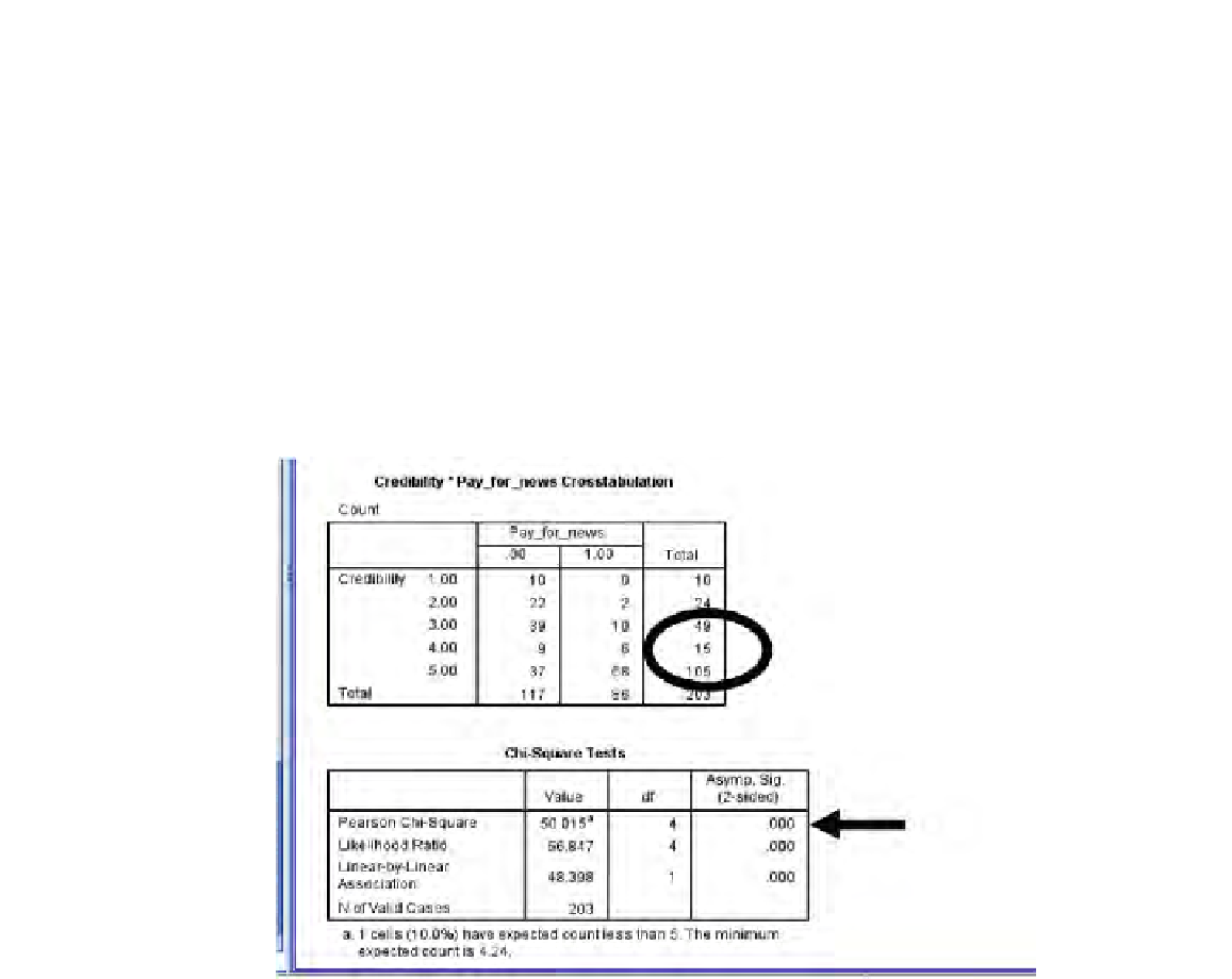
Figure 11.15 that about 83% (a total of 169, the sum arrived at by adding the individ-
ual numbers contained in the black oval in Figure 11.15 ) of the respondents indicated
that strong credibility was at least “3” on the 1-5 scale (1 = not at all impactful, 5 =
extremely impactful) in a decision to pay for an online news experience.
We now perform and discuss the binary logistic regression analysis. The output
is displayed in Figure 11.16 . 2
First, observe the “pseudo- R -square” values at the top of the igure. The Cox &
Snell R Square is 0.523 and the Nagelkerke R Square is 0.703. If we were to interpret
the Nagelkerke R Square as an r 2 value in a regular multiple linear regression, the 0.703
would indicate that we estimate that about 70% of the variability in Y (whether or not
a person would pay for some type of online news experience) is associated with the
variables in the equation. In loose terms, we estimate that these 13 X variables explain
70% of whether a person answers “Yes” or “No” to the question. So far, so good.
FIGURE 11.15
Chi-square test for strong credibility versus willingness to pay for online news; SPSS with
CharlestonGlobe.com.
2 The formal process for performing this analysis indicates that you should take steps to tell SPSS
which of the X variables are (0,1) or “categorical”-type variables. We believe that this is best not done,
as long as you are very clear which category got a 1 and which got a 0, and that you understand that a
positive coeficient indicates that, everything else equal, a “1” for that X increases the probability that
Y = 1 and a “0” decreases this probability, and that it is the reverse if the coeficient of the X is negative.
We believe that identifying these details in SPSS adds more confusion than beneit.