Database Reference
In-Depth Information
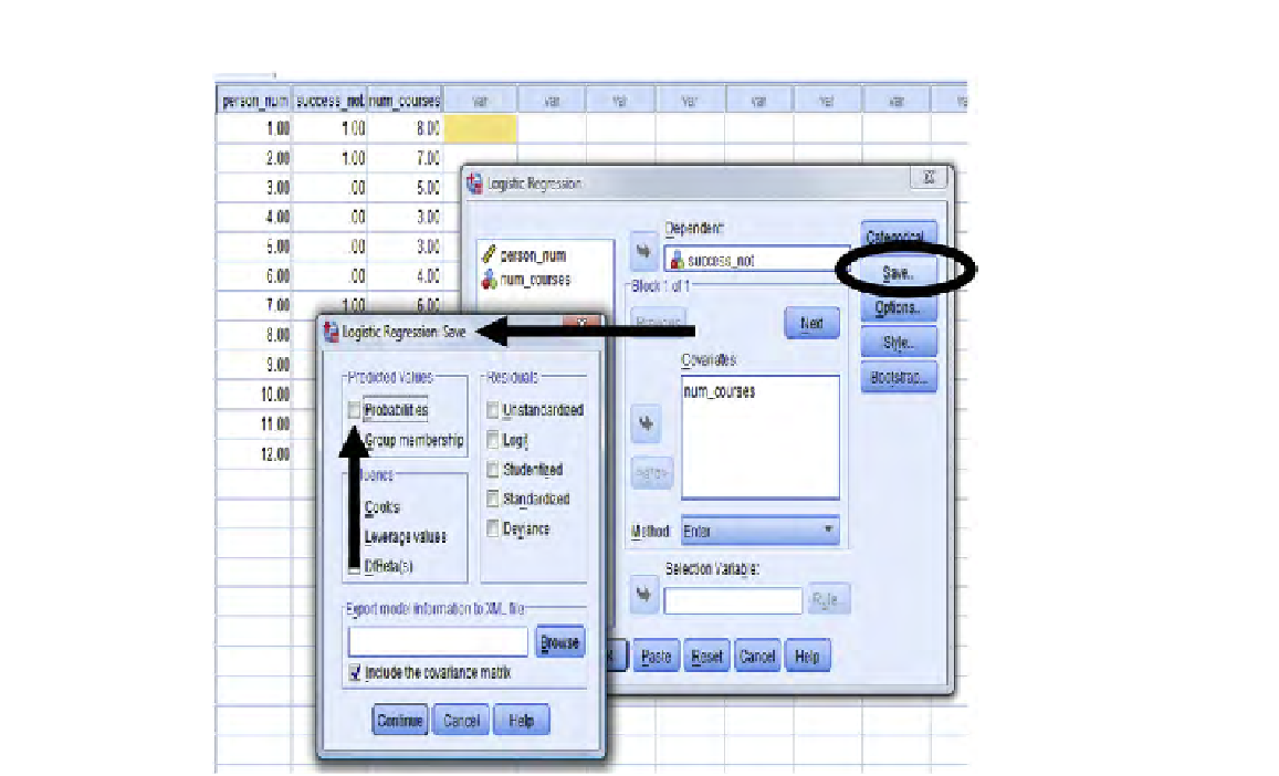
FIGURE 11.10
The Logistic Regression: Save dialog box; SPSS with illustrative example.
We now click on “Probabilities” in the top left part of the dialog box (see vertical
arrow in
Figure 11.10
). Now clicking “Continue” puts us back to
Figure 11.7
, where
we click “OK,” as we did earlier.
You can see in
Figure 11.11
that along with our three columns of original data, we
now have a new column, “PRE_1”—“prediction of a 1” (see oval in
Figure 11.11
).
This new column represents the predicted probability that each person will be a “1,”
or will successfully complete the task.
You can note that for row 1 of
Figure 11.11
, which has X (num_courses) = 8, you
see a probability of 0.95923. This is consistent with what we computed in the earlier
section as 0.96. For X = 5, which corresponds with both rows 3 and 8, the probability
is given as 0.15548, again, consistent with our result in the section of 0.16. In both
cases, the only difference is miniscule, involving rounding error.
You can see in
Figure 11.11
that we have obtained the predicted probability for
each X value in our data set. What if we want to predict the probability of a “1” for
a value of X that is
not in our data set
? How do we do that? Well, in the current
Search WWH ::

Custom Search