Can you relate? Correlation and simple linear regression - Improving the User Experience through Practical Data Analytics - page 223

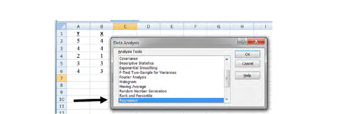
FIGURE 9.16
Regression command within data analysis; Excel with illustrative data.

To calculate this line, the vertical differences from the dots to the line are irst
squared and summed. For example, at X 1 , the line predicts 5, but the actual data value
equals 6, for a difference of 1. It can be proved that the least-squares line is unique.
In other words, there cannot be a tie for which line is the least-squares line. Perhaps
more importantly, Excel and SPSS will ind it for us.
First, let's begin by providing our notation 2 for the formula for a simple regres-
sion least-squares line:

Yc=a+b*X

where:
•

“Yc” is the predicted ( “c omputed”) value of Y based on a known value of X,

• “b” represents the slope of the line,

• “a” represents the intercept, or the point at which the line crosses the Y-axis

(sometimes called the “Y-intercept”).

There are some very tedious mathematical formulas you can use to calculate
the slope and intercept of the least-squares line (sometimes called the “regression
line”), but both Excel and SPSS will save you lots of time and headaches. Let's start
with Excel.

9.4.1 EXCEL
To do a regression analysis in Excel (and what we have been doing for all statistical
analyses in Excel) we irst open “Data Analysis.” Then, we scroll down to “Regres-
sion.” See Figure 9.16 , with the arrow pointing to the command.

2 There is no standard notation for this least-squares line. If you looked at 10 statistics/predictive
analytics/data analysis texts, you might see ive or six different notations for the slope and intercept.