Database Reference
In-Depth Information
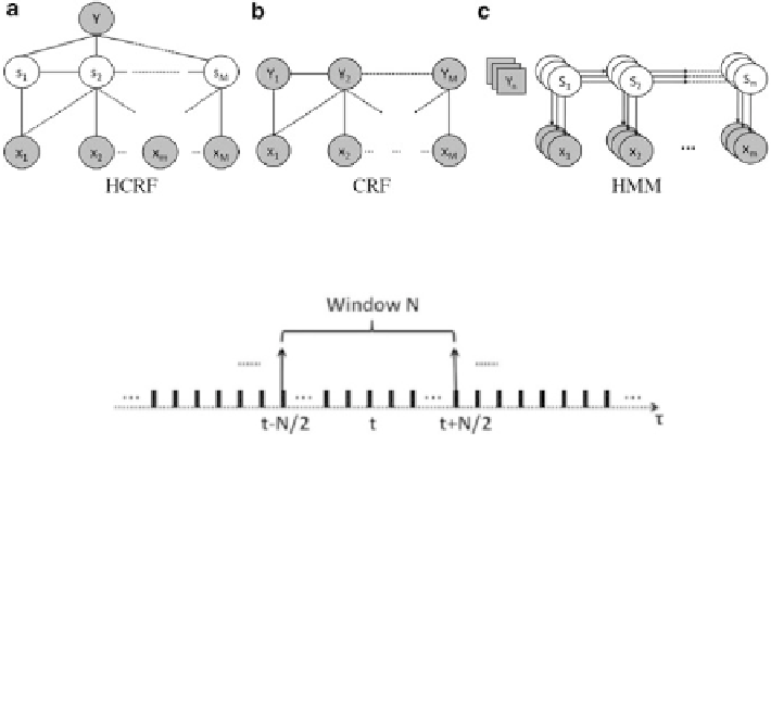
Fig. 9.4
Structured prediction models: (
a
) hidden conditional random field (HCRF); (
b
) condi-
tional random field (CRF); (
c
) hidden Markov model (HMM)
Fig. 9.5
HCRF input shown in Eq. (
9.7
), by sliding window average result on view types of
decoded image sequence
motion descriptor, introduced by Tan et al. [
296
]. The formula to calculate the
average values at time-stamp t are given in Eq. (
9.7
), where individual frame-based
probabilities are
p
s
j
=
1
,
2
,
3
,
4
and
p
c
.
t
+
N
/
2
1
N
∑
p
ws
j
(
t
)=
p
s
j
(
˄
)
with j
=
1
,
2
,
3
,
4
˄
=
t
−
N
/
2
t
+
N
/
2
∑
1
N
p
wc
(
t
)=
p
c
(
˄
)
(9.7)
˄
=
t
−
N
/
2
A label and training sequence pair is defined as
(
y
i
,
X
i
)
with the index number
i
x
i
,
M
are the event
label and observed states as Fig.
9.4
a depicts. For instance,
x
i
,
m
is interpreted
as the
m
th
=
1
,
2
,...,
n
. For each pair,
y
i
∈
Y
and
X
i
=
x
i
,
1
,
x
i
,
2
,
x
i
,
m
,...,
sampled time state of the
i
th
training sequence, where
x
i
,
m
(
t
)=
[
p
i
,
ws
1
(
t
)
,
p
i
,
ws
2
(
t
)
,
p
i
,
ws
3
(
t
)
,
p
i
,
ws
4
(
t
)
,
p
i
,
wc
(
t
)]
.
k
and
k
need to be learned. As Eq. (
9.6
)
During HCRF training, parameters
ʸ
ʸ
k
are coefficients for the state feature function
f
k
, which contains
a single hidden state, and the transition feature function
f
k
, which involves two
adjacent hidden states, respectively. In order to find the optimal parameters, a log-
likelihood objective function is used, as shown in Eq. (
9.8
), with a shrinkage prior
(the second term in the equation) in order to avoid the excessive parameter growth.
A limited-memory version of the Broyden-Fletcher-Goldfarb-Shanno (L-BFGS)
quasi-Newton gradient ascent method [
297
] is applied to find the optimal
k
and
shows,
ʸ
ʸ
ʸ
∗
=
Search WWH ::

Custom Search