Detecting distorted and benign blood cells using the Hough transform based on neural networks and decision trees - Emerging Trends in Image Processing, Computer Vision, and Pattern Recognition - page 386

3 Hough transforms
The Hough transform is a popular feature extraction technique that converts an image from
Cartesian to polar coordinates. Any point within the image space is represented by a sinus-
oidal curve in the Hough space. In addition, two points in a line segment generate two curves,
which are overlaid at a location that corresponds with a line through the image space. Even
though this model form is very easy, it is deeply complicated for the case of complex shapes
due to noise and shape imperfection, as well as the problem of finding slopes of vertical lines.
The CHT solved this problem by puting a transformation of the centroid of the shape in the
x-y plane to the parameter space [ 13 ] .
There are three essential steps common to all CHTs. First, a CHT contains an accumulator
array computation of high gradient foreground pixels, which chosen as candidate pixels. Then
they are collected “votes” in the accumulator array. Center estimation is the second step. It
predicts the circles centers by detecting the peaks in the accumulator array that produced
through voting on candidate pixels. The votes are accumulated in the accumulator array box
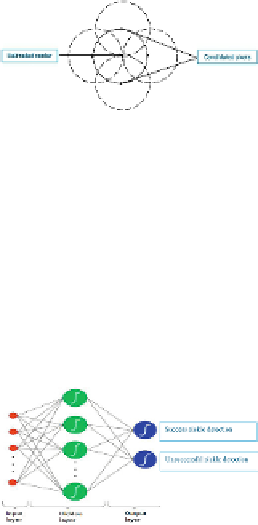
according to a circle's center. Figure 3 shows an example of the candidate pixels (solid dots)
falling on an actual circle (solid circle), as well as their voting paterns (dashed circles), which
coincide with the center of the substantial circle. The third step in a CHT is radius estimation;
if the same accumulator array has been used for more than one radius value, as is commonly
done in CHT algorithms, the radii of detected circles must be estimated as a separate step [ 2 ].
The radius can be clearly estimated by using radial histograms; however, in phase-coding, the
radius can be estimated by simply decoding phase information from the estimated center loc-
ated within an accumulator array [ 2 ] . For this chapter, I have used a CHT to detect and count
RBCs, even if they are hidden or overlapped. Watershed and morphological functions are used
to enhance and separate overlapped cells during the segmentation process.
FIGURE 3 Circle center estimated.
4 Overview of NN
Now, NN with back propagation is the most popular artificial NN construction, and it is
known as a powerful function approximation for prediction and classification problems. His-
torically, the NN has been viewed as a mutually dependent group of artificial neurons that
uses a mathematical model for information processing, with a connected approach to compu-
tation introduced by Freeman in 1991 [ 4 , 14 ] . The NN structure is organized into layers of in-
put, output neurons, and hidden layers, as in Figure 4 .
FIGURE 4 The structure of a neural network.