Global Positioning System Reference
In-Depth Information
20
15
10
5
0
−5
−10
−15
2
4
6
8
10
12
14
16
18
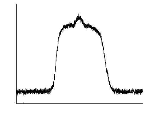
Frequency [Mhz]
FIGURE 4.6. Frequency domain. Representation of 1,048,576 samples of GPS L1 data.
the histogram. Also the histogram bears a strong resemblance to the probability
density function for a Gaussian random variable, which would be expected for
white thermal noise. These plots follow what would be expected based on the fre-
quency domain depiction in Figure 4.1 where the thermal noise would dominate
the resulting samples.
However, the frequency domain depiction does not resemble Figure 4.1; rather
some obvious structure is present. This structure is best explained by building on
Figure 4.1, as shown in Figure 4.7.
In this figure, obvious changes have been made to better correspond to the
frequency domain depiction of the collected data file.
First, the “noise level” is not white, or flat and uniform as a function of fre-
quency, but has some definite structure. This is a result of the final bandpass filter
prior to sampling. This 6 MHz-wide bandpass filter shapes the spectrum of the
analog signal to be sampled. Thus, the filter shape has been added within Fig-
ure 4.7.
Second, there is an obvious “bulge” within the center of the passband right at
the resulting IF of the GPS translated signal. This actually appears to be the main
2
046 MHz lobe of the sinc spectrum of the signal itself. With the specified re-
ceived signal power level so much lower than the expected thermal noise, how can
there be any discernable structure from the satellite signal from a data set collected
with a traditional hemispherical antenna? The explanation has two components:
.
-
the individual received satellite signal power is currently higher than the
minimum specified (as shown in Figure 4.7); and
-
the CDMA nature of the GPS system has all the satellite signal power over-
laid at the resulting IF; thus, the spectrum shows the summation of all the
visible satellite signal power.


Search WWH ::

Custom Search