Statistical Methods - Text Mining Techniques for Healthcare Provider Quality Determination - page 76

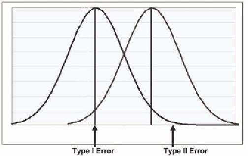
Figure 1. Difference in two curves

H 0 : μ= μ 0 , the effect size is equal to 2

s

n - , where s is the sample standard deviation and n is the
sample size. Note that as n increases, the value of 2

1

s

n - decreases so that the effect size begins to 1

converge to zero.
Consider a simple example. The heartbeat of unborn girls tends to be higher than for unborn boys.
Then Figure 1 demonstrates the situation of testing the hypotheses:

H 0 : infant is a girl
H 1 : infant is a boy

Each infant is a sample of size 1. The curve to the left represents the possible heartbeats for the
boys; the curve to the right is for girls. We can reject the null hypothesis if the heartbeat is lower than
the leftmost line in the Figure. The amount of the right curve that is to the left of that line represents the
Type I error, the probability that the infant is a girl. Similarly, the amount of the left curve that is to the
right of the rightmost line is the Type II error. The effect size is the distance between the two curves.
It represents the portion of the curve where no decision about H 0 and H 1 can be made. In this example,
since there is only one observation, the observation is equal to the sample mean. Increasing the sample
size while holding the Type I and II errors fixed will decrease the effect size. However, it must be re-
membered that the effect size will only decrease when considering the average; any individual subject
can vary considerably more than the mean.
Suppose, for example, that we want to determine whether patients with diabetes have a longer length
of hospital stay and higher total charges compared to patients without diabetes. We can use different
sample sizes from the National Inpatient Sample to examine this hypothesis H 0 : μ 1 = μ 2 where group
1=patients with diabetes and group 2=patients without diabetes. With a sample of size 50 for an unpaired
t-test, we get the result that the difference is not statistically significant. The confidence interval for the
difference in the length of stay is (-1.819, 2.2194) and for total charges is equal to (-16,438, 6299.50).
These are quite large and include the value of zero, the null hypothesis.
To compute a sample that is stratified proportionally to the occurrence of diabetes, we use the fol-
lowing SAS code: