The All Patient Refined Diagnosis Related Group - Text Mining Techniques for Healthcare Provider Quality Determination - page 208

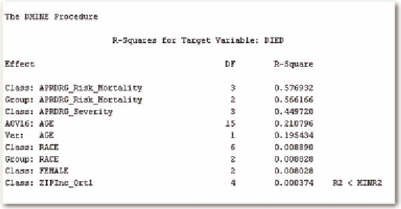
Figure 4. Results of Dmine regression

Y =+ + ab g X Z

where α is equal to the intercept and β is the coefficient of the patient demographic information. The
coefficient, γ, is multiplied by the value of Z, the APRDRG index. Then we have

ì

ï ï ï ï ï ï

g
g
g
g

if APRDRG
if APRDRG
if APRDRG
if APRD

=
=
=

1

2 2

Y =+ + ab X

í

ï ï ï ï ï ï 3 3

4 RG = 4

î

Therefore, as the index increases, so does the predicted value, Y. However, the actual model is slightly
more complicated in that α+βX also increases the value of Y, but at a fixed value independent of the value
of the APRDRG index. It will be more complicated, still, if we use both the APRDRG mortality and
severity indices in the model. In order to ensure the lack of multicollinearity, we first examine the cor-
relation of the two indices, which is 72%. It is high, so we will see if the model is relatively accurate. We
first use logistic regression to examine the predicted mortality. The odds ratios are given in Table 3.
The odds ratios indicate that all of the variables are statistically significant. There is a 91% accuracy
level. The receiver operating curve is given in Figure 1, with a c statistic of 0.928; the c statistic gives
the area under the ROC curve.
Table 4 gives the classification table. It shows that there is a problem when examining false positives
versus false negative rates. The false negative rate is over 50% while the false positive rate is extremely
small.
We contrast the logistic regression as performed in the traditional statistical manner to that of predic-
tive modeling. In this approach, we sample a 50/50 split in the data to account for the rare occurrence.
Then we partition the data to find the optimal sample. We use multiple methods including regression,
decision trees, and neural networks. We also examine the lift to see if part of the data can be predicted