Graphics Reference
In-Depth Information
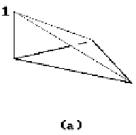
Figure 19.6.
Local triangle and quadrilateral shape functions.
for H(x) were the T
i
and we found those by solving a system of linear equations (19.14),
which is straightforward.
Two-dimensional applications of the FEM proceed in essentially the same way.
The main difference is that the differential equations get more complicated. Figure
19.6 shows some linear two-dimensional local shape functions for triangular and
quadrilateral elements. Again, these functions, whether they are linear or not, have
the property that they vanish at all nodes except one.
19.5
Summary
We end with some general comments. The FEM is important because most real-world
problems are too complex to be solved in closed form. It is a very successful method
for solving nonlinear differential and integral equations numerically. The approxima-
tions are based on local shape functions, typically polynomials, for elements whose
solutions are specified by data at their nodes. This involves a choice of local shape
functions and a mesh. The accuracy of the solutions is measured with respect to some
suitable choice of definition for the distance between functions. Common distance
functions are based on the L
p
norms || ||
1
, || ||
2
, and || ||
•
(see Section 21.4 for a defi-
nition). Although these are usually not easy to compute, one can find approximations
to them. Rectangular or triangular meshes are common and one often uses adaptive
meshes that change in size and are not uniform over the entire region of interest.
Getting good meshes is very important because numeric accuracy suffers otherwise,
for example, if triangles are skinny and have very large or small angles. So-called
multi-grid methods have provided some of the fastest solutions.
The basic steps in the FEM approach are:
(1) Find the equations that govern the physical phenomenon.
(2) Replace these equations with their “weak” formulation.
(3) Subdivide the domain into appropriate elements and decide on the basis func-
tions to use for each element.
(4) Combine the individual element solutions into a global solution according to
the Galerkin approximation to obtain global matrix equations.
(5) Solve these matrix equations using the given boundary conditions.