Graphics Reference
In-Depth Information
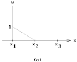
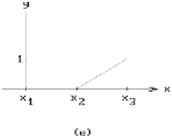
Figure 19.5.
Local and global shape functions.
element would not work since the function would not be differentiable at the nodes
and have zero second derivative on the interior of the elements. To get around this
problem we need to reformulate (19.10). One can show, using integration by parts,
that (19.10) is equivalent to
L
K
dw
dx
dT
dx
dx
dT
dx
L
L
È
Í
˘
˙
Ú
Ú
()
()
-
w x Qdx
-
Kw x
=
0
.
(19.11)
0
0
0
The advantage with (19.11) is that only the first derivative is involved. Equation (19.11)
is called the
weak form of the one-dimensional heat flow equation
. The term “weak” is
used because there is less of a differentiability requirement. Using linear approxima-
tions no longer causes a problem.
The next step is to decide how many elements we want to create. Suppose that
we use two. We also have to decide on basis functions. We shall use linear functions,
in fact, the linear B-splines or hat functions discussed in Section 11.5. See Figure
19.5(a). For an arbitrary interval [a,b], any linear functions h(x) can be expressed as
linear combinations of the two functions
()
=-
-
-
xa
ba
and
xa
ba
-
-
()
=
=-
()
bx
1
b
x
1
bx
,
a
b
a
namely,
()
=
() ()
+
() (
.
hx
hab x
hbb x
a
b
See Figure 19.5(b). The functions b
a
(x) and b
b
(x) are the
local
(linear) shape function
basis for the interval [a,b]. Using functions like this we associate a global shape func-