Graphics Reference
In-Depth Information
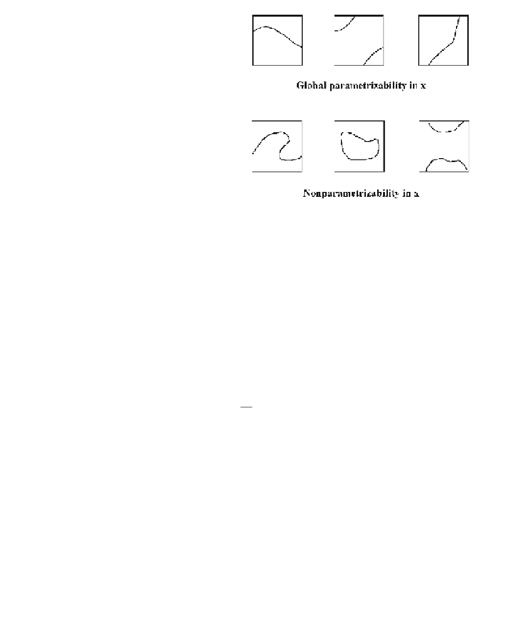
Figure 18.3.
Parameterizability in x.
to do so essentially means that the set defined by the equation can be represented as
the graph of a function locally. [Snyd92] defines a curve to be
globally parameterizable
in the ith coordinate
in a proximate interval if no two distinct points of the curve in
the interval have the same ith coordinate. See Figure 18.3. He gives an interval version
of the implicit function to be used for testing for that condition. He also describes a
heuristic test for this condition that avoids expensive computations with Jacobians.
In Example 18.5.1 we have global parameterizability in the y-coordinate because
∂
∂
f
y
=10.
We also have it in the x-coordinate, but because
∂
∂
f
x
=-2
x
vanishes when x is 0, we do not get this fact entirely from the implicit function
theorem. The way that this condition gets used in Algorithm 18.5.1 is that when it
holds, only adjacent pairs of points are connected by curve segments after the points
of intersection of the curve with the boundary of a proximate interval are ordered by
the ith coordinate. For Step 3 we need assumption (2) in the algorithm. By tagging
edges appropriately we can arrange it so that a computation is done only once for
each edge (not once for each of the two adjacent intervals, or four in the case of a
corner). See Figure 18.4. The disjointness of the intervals achieved in Step 4 is needed
to sort them. We need this ordering in Step 5.
Finally, [Snyd92] describes ways to relax the assumptions needed for Algorithm
18.5.1, namely, the assumption that the curve is nonsingular, that it have no endpoints
in the interior of proximate intervals, and that it is transverse to boundaries of
intervals.